Microeconomics and Macroeconomics

This lecture provides mathematical models to reason about economics in the small (microeconomics) and about economics in the large (macroeconomics).

Supply, Demand, Elasticity

Consider a market of a single commodity with many producers and many consumers. We define the supply and the demand functions.

Definition of the demand function.

The demand function \(q = D(p)\) gives the quantity \(q\) of units that will sell at price \(p\).

Naturally, demand decreases with increasing price.

Definition of the supply function.

The supply function \(q = S(p)\) gives the number of units that all producers will supply at price \(p\).

Naturally, supply increases with increasing price.

Consider a numerical example, with demand \(D(p) = 2/p\) and supply \(S(p) = p - 1\), as shown in Fig. 59.

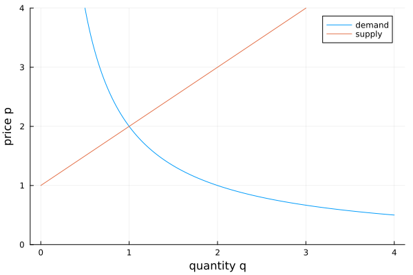
Fig. 59 A numerical example of a supply and demand function.

Traditionally, the quantity \(q\) appears on the horizontal axes, so we plot \(D_q(q) = 2/q\) and \(S_q(q) = 1 + q\).

We find the equilibrium price where supply and demand intersect, as shown for an example in Fig. 60.

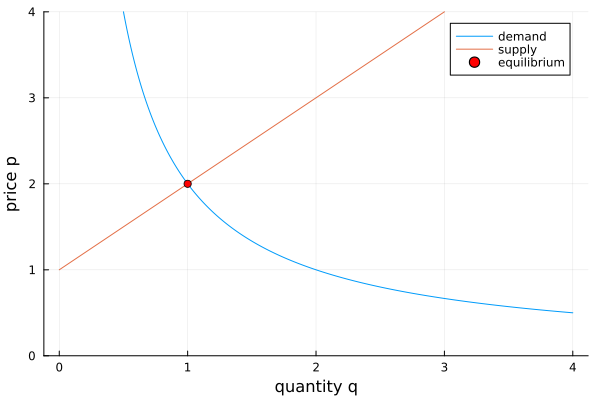
Fig. 60 A numerical example of the equilibrium price.

Definition of the equilibrium price.

Given demand \(D(p)\) and supply \(S(p)\), the equilibrium price \(p_0\) is the intersection of demand and supply:

\[D(p_0) = q_0 = S(p_0).\]

Prices naturally converge to the equilibrium.

• At prices above the equilibrium, more goods will be produce than the market can absorb and this surplus drives down prices.

• At prices below the equilibrium, when demand is higher than the supply, this scarcity will lift prices upwards.

What is the effect of a sales tax?

• Supply remains, because the consumer pays the tax.

• What is the new demand function?

The consumer pays \(p (1 + T)\), where \(T\) is the tax, e.g.: \(T = 10\%\). The new demand function is therefore

\[q = D_T(p) = D(p + Tp),\]

where \(D(p)\) is the original demand, before the tax. Therefore, a sales tax of \(10\%\) depresses demand. Returning to our numerical example from before, for \(D(p) = 2/p\), the new demand is \(D(p + Tp) = 2/(p+Tp) = q\), shown in Fig. 61. Observing that \(q\) is displayed on the horizontal axis, plotting \(p\) in function of \(q\), we use \(D_q(q) = 2/(q(1+T))\).

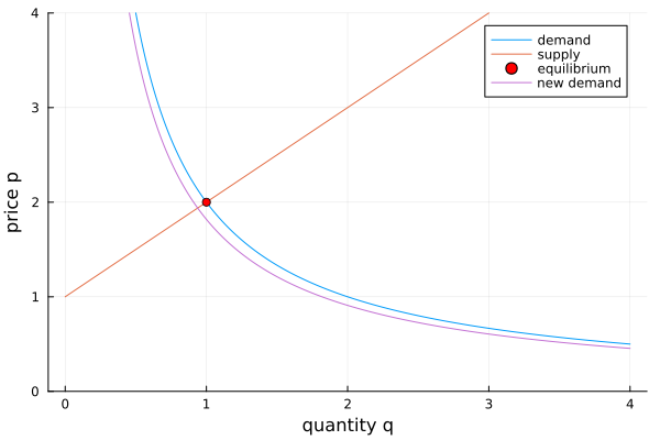
Fig. 61 The effect of a \(10\%\) sales tax on the consumer.

It is an exercise to consider the effect of a tax on the producer.

Given supply and demand, we next define revenue, cost, and profit.

Definition of revenue.

The revenue of a producer \(R(p,q)\) equals \(p \cdot q\), the quantity \(q\) sold times the price \(p\) received for each unit sold.

At the equilibrium price \(p_0\), the revenue is \(R(q) = p_0 q\).

Definition of cost.

The cost of a producer \(C(q)\) is the cost to produce \(q\) units which includes the fixed cost equal to \(C(0)\).

The cost function increases with \(q\) and tends to flatten.

Definition of profit.

The profit of a producer \(P(q) = R(q) - C(q)\), revenue minus cost.

A geometric interpretation of revenue views revenue as an area, shown in Fig. 62.

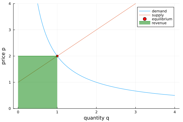
Fig. 62 The revenue \(R(p,q) = p \cdot q\) as area.

What is the effect of a sales tax on revenue? Recall the effect of a sales tax.

1. The sales tax depresses the demand.

2. The quantity sold decreases.

3. The equilibrium price drops.

Consequently, the revenue \(R(p,q)\) decreases. The public sector revenue from a sales tax \(T\) is

\[G(p,q) = T \cdot p \cdot q.\]

Next we define marginal cost and marginal revenue.

Definition of marginal cost.

The marginal cost is the additional cost to produce one more unit.

For the cost function \(C(q)\) we have

\[\frac{C(q+1) - C(q)}{1} \approx C'(q).\]

Definition of marginal revenue.

The marginal revenue is the additional revenue from one more unit.

The importance on marginal profit and marginal cost is summarized by the following theorem.

Theorem on optimal profit.

Profit is optimal when \(R'(q) = C'(q)\).

To illustrate the theorem, we consider a numerical example. Revenue \(R(q)= 5q\) while cost is \(C(q) = 4 + q^2\), illustrated in Fig. 63.

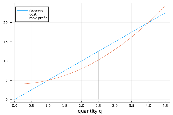
Fig. 63 Revenue, Cost, and maximum profit.

From Fig. 63, we see that maximum profit happens when \(R'(q) = 5 = 2q = C'(q)\), at \(q = 2.5\).

To arrive at elasticity of demand, consider the following question. By how much can a producer raise the price of a product?

\[R(p,q) = p \cdot q, \quad \mbox{as} \quad q = D(p), \quad \mbox{we have} \quad R(p,q) = p \cdot D(p).\]

What is the change in demand as the price changes?

Definition of elasticity of demand.

The elasticity of demand \(e\) is

\[e = - \frac{\mbox{change in demand}}{\mbox{change in price}}.\]

The sign of \(e\) is negative as demand decreases for increasing price.

We next derive an expression of the elasticity.

\[\begin{split}\begin{array}{rcl} e & = & {\displaystyle - \frac{\mbox{change in demand}} {\mbox{change in price}}} \\ & = & {\displaystyle - \frac{dq/q}{dp/p}} \\ & = & {\displaystyle - \frac{dq}{dp} \cdot \frac{p}{q}}, \quad q = D(p), \quad dq = D(p+dp) - D(p) \\ & = & - p \left( \frac{1}{D(p)} \right) \left( \frac{D(p+dp) - D(p)}{dp} \right) \end{array}\end{split}\]

Theorem on the elasticity as a function of price.

\[e = - p \frac{D'(p)}{D(p)}\]

What is the change in revenue as the price changes? Let us derive revenue as a function of elasticity.

\[\begin{split}\begin{array}{rcl} {\displaystyle \frac{dR}{dp}} & = & {\displaystyle \frac{d}{dp} \left( \vphantom{\frac{1}{2}} p \cdot D(p) \right)}, \quad \mbox{as} \quad R(p,q) = p \cdot D(p) \\ & = & 1 \cdot D(p) + p \cdot D'(p) \\ & = & {\displaystyle D(p) \left( 1 + p \frac{D'(p)}{D(p)} \right)}, \quad e = - p \frac{D'(p)}{D(p)} \\ & = & D(p) (1 - e) \end{array}\end{split}\]

The change in revenue in function of demand and elasticity:

\[\frac{dR}{dp} = D(p) (1 - e).\]

Let us do a case analysis:

• \(e > 1\): revenue decreases when price increases. We then say that the demand is elastic.

• \(e < 1\): revenue increases when price increases. We then say that the demand is inelastic.

• \(e = 1\): implies \(\displaystyle \frac{d R}{d p} = 0\), optimal revenue.

This analysis determines the price setting in a monopoly.

An exercise asks to consider elasticity for a linear demand function.

Duopolistic Competition and Price Dynamics

In microeconomics, we consider only one producer. Now we consider two competing producers, going to a larger scale, into macroeconomics. We make two assumptions.

1. The demand function is the same for both producers. For example, bottled water.

2. Each producer believes the other will hold its output constant. This model was proposed by Cournot in 1838.

What is the price setting mechanism?

To formalize the price dynamics, we introduce some notation. The competitors \(A\) and \(B\) have the same demand \(q = D(p)\).

1. Assume \(A\) is alone on the market at first. \(A\) sets the price according to elasticity \(e = 1\):

   \[p = a_1 = - \frac{D(a_1)}{D'(a_1)}.\]

2. \(B\) enters, the demand is decreased with \(q_A = D(a_1)\). The demand function for \(B\) is then \(D(p) - D(a_1)\). \(B\) sets the price according to elasticity \(e = 1\):

   \[p = b_1 = - \frac{D(b_1) - D(a_1)}{D'(b_1)}.\]

Now we will be deriving a discrete time system. Rewrite

\[b_1 = - \frac{D(b_1) - D(a_1)}{D'(b_1)}\]

as

\[D'(b_1) b_1 + D(b_1) = D(a_1).\]

Now \(A\) reacts to the new demand curve \(D(p) - D(b_1)\):

\[a_2 = - \frac{D(a_2) - D(b_1)}{D'(a_2)},\]

which can be rewritten as

\[D'(a_2) a_2 + D(a_2) = D(b_1).\]

A discrete time system emerges. Assuming \(A\) is leader and \(B\) is follower, we start with

\[a_1 = - \frac{D(a_1)}{D'(a_1)},\]

and continue for \(k = 1,2 \ldots\) with

\[D'(b_k) b_k + D(b_k) = D(a_k)\]

and

\[D'(a_{k+1}) a_{k+1} + D(a_{k+1}) = D(b_k).\]

This can be formulated as a fixed-point iteration, converging to an equilibrium if the equations are contractive.

The Cobb-Douglas Model of Production

The Cobb-Douglas model expresses production \(Q\) as a function of

• \(L\), labor, and

• \(K\), capital investment

where \(A\) is some constant depending on technology:

\[Q = A ~ L^\alpha K^{1-\alpha}, \quad 0 < \alpha < 1.\]

Note that \(Q = Q(L,K)\) is homogeneous. For some \(\lambda > 1\):

\[\begin{split}\begin{array}{rcl} Q(\lambda L, \lambda K) & = & A ~ (\lambda L)^\alpha (\lambda K)^{1-\alpha} \\ & = & A ~ \lambda^\alpha L^\alpha \lambda^{1-\alpha} K^{1-\alpha} \\ & = & A ~ \lambda L^\alpha K^{1-\alpha} \\ & = & \lambda Q(L, K) \end{array}\end{split}\]

For example: doubling labor and capital doubles the output.

What is the effect of the addition of one extra unit of labor? This question leads to the notion of marginal product of labor. Take the derivative of \(Q\) with respect to \(L\):

\[w = \frac{d Q}{d L} = A \alpha L^{\alpha-1} K^{1 - \alpha} = \alpha \frac{Q}{L}\]

is the marginal product of labor, which should equal the wage \(w\) paid to a worker.

What is the effect of the addition of one extra unit of capital? This question leads to the notion of marginal product of capital. Take the derivative of \(Q\) with respect to \(K\):

\[r = \frac{d Q}{d K} = A (1 - \alpha) L^{\alpha} K^{1 - \alpha - 1} = (1 - \alpha) \frac{Q}{K}\]

is the marginal product of capital, which should equal the rent \(r\) for capital.

Expressing production \(Q\) in function of labor \(L\) and capital \(K\):

\[Q = A ~ L^\alpha K^{1-\alpha}, \quad 0 < \alpha < 1, \quad w = \alpha \frac{Q}{L}, \quad r = (1 - \alpha) \frac{Q}{K}.\]

Observe

\[L w + K r = \alpha Q + (1-\alpha) Q = Q,\]

independent of the technology \(A\). So, we derived a macroeconomic law:

Theorem, the Cobb-Douglas model.

\[Q = w L + r K\]

In words, production is the sum of

1. marginal product of labor times labor, and

2. marginal product of capital time capital investment.

As a microeconomic application, consider the following. For a specific product made by a producer, determine in

\[Q = A ~ L^\alpha K^{1-\alpha}, \quad 0 < \alpha < 1.\]

the parameters \(A\) and \(\alpha\) by sampling and fitting. Then apply the formula \(Q = w L + r K\) as follows.

To increase production,

1. hire more workers if \(w > r\), or

2. raise more capital if \(w < r\).

The Leontiev Input/Output Model

The Leontiev input/output model considers three sectors:

\[A : \mbox{ Agriculture} \quad I : \mbox{ Industry} \quad S : \mbox{ Service},\]

each producing \(x_1\), \(x_2\), \(x_3\) goods respectively. \(C\) is the demand of the Consumer sector. The equation

\[x_1 = 0.3 x_1 + 0.2 x_2 + 0.3 x_3 + 4\]

expresses that for all goods produced by Agriculture

1. \(30\%\) is consumed by Agriculture,

2. \(20\%\) is consumed by Industry,

3. \(30\%\) is consumed by Service,

and the remaining 4 units are absorbed by the Consumer sector.

The three equations

\[\begin{split}\begin{array}{rcl} x_1 & = & 0.3 x_1 + 0.2 x_2 + 0.3 x_3 + 4 \\ x_2 & = & 0.2 x_1 + 0.4 x_2 + 0.3 x_3 + 5 \\ x_3 & = & 0.2 x_1 + 0.5 x_2 + 0.1 x_3 + 12 \end{array}\end{split}\]

can be summarized into a single matrix relation

\[{\bf x} = A {\bf x} + {\bf b}.\]

The vector \(\bf b\) is called the bill of goods. Then the question is Is the bill of goods realizable? The question is equivalent to asking whether

\[{\bf x} = A {\bf x} + {\bf b}\]

has a solution with all entries in \(\bf x\) positive. The solution is \({\bf x} = (I-A)^{-1} {\bf b}\). The series expansion of \((I-A)^{-1}\) is

\[\frac{1}{I - A} = I + A + A^2 + \cdots\]

which converges only if \(\|A\|_2 < 1\), if the dominant eigenvalue is less than one in modulus.

Proposals of Project Topics

1. Nash equilibria.

   The concept of a Nash equilibrium is important in game theory. Read the Game Theory book of Hans Peters for the definition and provide a computational description of a good example.

   Consider the following questions.

   1. Formulate an economically interesting model.

   2. Give an example of an application with many Nash equilibria.

2. Model a price war.

   Develop a computational model of a price war. Read chapter 11 of It’s a Nonlinear World by Richard Enns.

   Consider the following questions.

   1. Formulate a model with a plausible demand function.

   2. Is it possible that chaos occurs?

Exercises

1. Consider \(S(p) = 20 p - 50\) and \(D(p) = 100 - 30p\). Suppose the producer must pay a specific tax of \(\$1\) per unit.

   1. What is the before tax equilibrium price?

   2. What is the after tax equilibrium price?

   3. How much of the tax is then actually paid by the consumer?

2. Consider a linear demand function, represented by \(D(p) = q_0 - m p\).

   1. Compute the elasticity \(e\).

   2. For which price \(p\) is \(e = 1\)?

3. Consider the duopolistic competition for a linear demand function, represented by \(D(p) = q_0 - m p\).

   1. Verify that the model converges.

   2. What is the equilibrium price?

Bibliography

1. Richard H. Enns: It’s a Nonlinear World. Springer Undergraduate Texts in Mathematics and Technology, 2011. Chapter 11 describes nonlinear models of competition.

2. Charles R. MacCluer, Chapter 8 of Industrial Mathematics. Modeling in Industry, Science, and Government, Prentice Hall, 2000.

3. Hans Peters: Game Theory. A Multi-Leveled Approach. Springer 2008. Page 7 gives an example of a Cournot game.