Supervised and Unsupervised Learning
We start by defining machine learning, then introduce the k-means algorithm to classify data in clusters. The next technique is principal component analysis to reduce the dimension of data. We end by summarizing the training and testing method.
Definitions
There is not a clear boundary between statistics and machine learning is a quote taken from Chapter 9 on Machine Learning Basics in Statistics with Julia. Fundamentals for Data Science, Machine Learning and Artificial Intelligence a book by Yoni Nazarathy and Hayden Klok, Springer 2021.
A popular quote from computer scientist Tom Mitchell provides as a workable definition for machine learning.
The quote above is taken from the following book: Gavin Hackeling: Mastering Machine Learning with scikit-learn. Apply effective learning algorithms to real-world problems using scikit-learn. Packt publishing, 2014.
We distinguish between two types of machine learning:
Supervised learning: given are labeled inputs and outputs, the program learns from examples of the right answers.
Unsupervised learning: the program does not learn from labeled data.
Two most common supervised machine learning tasks are classification and regression. Examples of unsupervised learning are clustering and dimensionality reduction.
An example of supervised learning is about finding distinctive elements in images. Consider Fig. 64. The pictures are copied from What Makes Paris Look Like Paris? by Carl Doersch, Saurabh Singh, Abhinav Gupta, Josef Sivic, and Alexei A. Efros in Communications of the ACM, Vol 58, No 12, pages 103-110, 2015.
Can we recognize the city from pictures taken in the city?
We know where each picture was taken.
So this is an example of index:supervised learning.
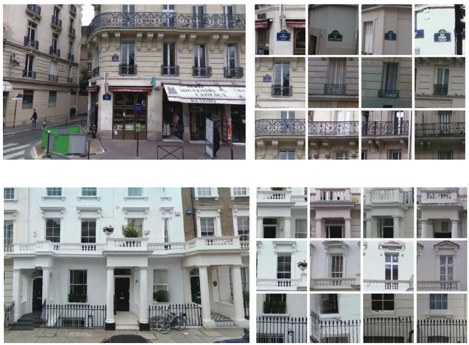
Fig. 64 Paris or London?
An example of unsupervised learning is predicting the value of a house. We are looking for a number.
The value of a house is it sales price.
If the house is not on the market, then there is no right answer.
So this is an example of unsupervised learning. In practice, we compare with recently sold houses in the neighborhood.
Clustering by the k-Means Algorithm
To illustrate the k-means algorithm, we introduce the Iris plants dataset, first used by Sir R. A. Fisher (1936). The problem is to classify plants given their attributes. This data is well known in the pattern recognition literature, used in statistics software such as R and in machine learning packages such as scikit-learn.
The Iris plants data is summarized below.
There are 150 instances, partitioned into three classes. We have 50 instances of each class with names
Iris-setosa,Iris-versicolor, andIris-virginica.Each instance has four attributes: sepal length and width, petal length and width (measured in cm). For the notions of sepal and petal, see Fig. 65.
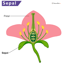
Fig. 65 Illustration of petal and sepal, image from SienceFacts.net.
We have features and labels:
The attributes of each plant are called features, represented by a 4-by-150 floating point matrix.
The names of the plants are called labels, represented by an array of 150 strings.
We can view features as input \(X\) and labels as output \(Y\).
In Julia, we load the Iris plants data as follows:
using MLDatasets: Iris

F, L = Iris(as_df=false)[:]
Then we have the data as follows:
The
Fis a 4-by-150 matrix ofFloat64elements.The
Lis a 150-element vector of elements of typeString.
Grouping the data into clusters is done by the index:k-means algorithm. The input to this algorithm is
\(L\) a list of points; and
\(k\) the number of centroids.
The steps in the algorithm are as follows:
\(C :=\) a random selection of \(k\) points of \(L\)
repeat
for each \(p \in L\):
if \(p\) is closest to \(C_i\), then put \(p\) in the i-th cluster
recompute the centroids for each of the \(k\) clusters
show the clusters
until the clusters are stable.
The k-means algorithm will be illustrated on the Iris plants data:
The features are in the 4-by-150 matrix
F.The labels are in the 150-element vector
L.
In Julia, we use the Clustering package.
using Clustering
C = kmeans(F, 3)
dump(C)
In the returned C.assignments we have 150 integers, 1, 2, or 3,
corresponding to the three computed centroids in the data.
The C.counts are [62, 50, 38], for one run.
In Fig. 66 and Fig. 67 are
the plots of the results of this one run.
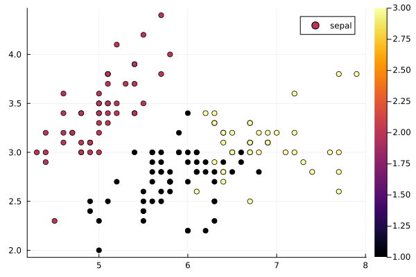
Fig. 66 Assignments plotted versus sepal data.
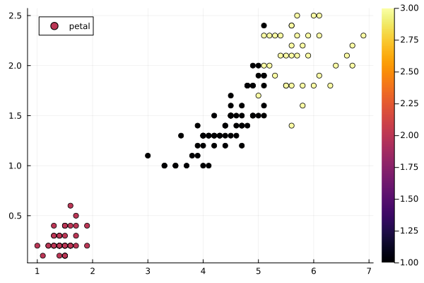
Fig. 67 Assignments plotted versus petal data.
Dimension Reduction via Principal Component Analysis
Principal Component Analysis (PCA) derives an orthogonal projection to convert observations to linearly uncorrelated variables, called principal components. Given a PCA model, we transform the observations \(x\)
into its principal components \(y\), with a projection matrix \(P\). The observations can be reconstructed from principal components:
In Julia, the principal component analysis
is available in the package MultivariateStats.
We distinguish three steps in the Principal Component Analysis:
Standardize the data, via the formula
\[z = \frac{x - \mbox{mean}}{\mbox{standard deviation}},\]applied to each number \(x\) in the input.
Setup the covariance matrix \(C\). For each pair \((z_i, z_j)\),
\[{\rm cov}(z_i, z_j) \mbox{ is the } (i,j)\mbox{-th element of the matrix.}\]The matrix \(C\) is symmetric and positive definite.
Compute the eigenvectors and eigenvalues of \(C\).
Sort the eigenvectors in increasing magnitude of the eigenvalues.
Then the feature vector consist of the first \(p\) eigenvectors.
The making of a PCA model is illustrated on the features
of the Iris data set.
The output of M3d = fit(PCA, F; maxoutdim=3) is
PCA(indim = 4, outdim = 3, principalratio = 0.99481691454981)

Pattern matrix (unstandardized loadings):
------------------------------------------
        PC1         PC2         PC3
------------------------------------------
1   0.743227   0.323137   -0.162808
2  -0.169099   0.359152    0.167129
3   1.76063   -0.0865096   0.0203228
4   0.737583  -0.0367692   0.153858
------------------------------------------

Importance of components:
-----------------------------------------------------------
                                PC1        PC2        PC3
-----------------------------------------------------------
SS Loadings (Eigenvalues)  4.22484   0.242244   0.0785239
Variance explained         0.924616  0.0530156  0.0171851
Cumulative variance        0.924616  0.977632   0.994817
Proportion explained       0.929434  0.0532918  0.0172747
Cumulative proportion      0.929434  0.982725   1.0
-----------------------------------------------------------
The PCA model M3d projects the 4-by-150 matrix F
onto a three dimensional matrix of points:
F3d = transform(M3d, F)
The data was sorted according to the plant class, so we plot the groups of 50 as follows:
scatter(F3d[1,1:50], F3d[2,1:50], F3d[3,1:50], label="setosa")
scatter!(F3d[1,51:100], F3d[2,51:100], F3d[3,101:150], label="versicolor")
scatter!(F3d[1,101:150], F3d[2,101:150], F3d[3,101:150], label="verginica")
The result of the above command is shown in Fig. 68.
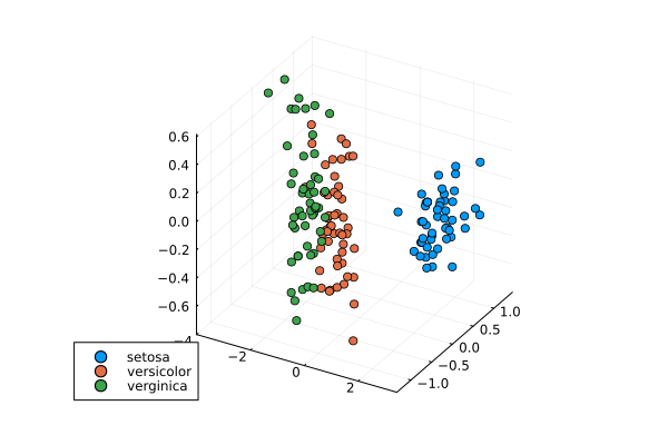
Fig. 68 The Iris data set reduced to three dimensions.
The training and testing method is summarized below. Learning in a supervised setting is a 2-step process:
Use one part of the data set to train the model.
Test the model on the other part of the data set.
Applied to the Iris plants data:
Train a model with the odd indexed features.
Test the model on the even indexed features.
With principal component analysis:
Train the PCA model using the odd indexed features.
Transform the even indexed features and reconstruct.
Proposals of Project Topics
Machine Learning with
scikit-learnGavin Hackeling: Mastering Machine Learning with scikit-learn. Apply effective learning algorithms to real-world problems using scikit-learn. Packt publishing, 2014.
One software that learns from experience is
scikit-learn.Read the book and the software documentation.
Describe how it fits in the computational ecosystem of Python.
Illustrate the capabilities by a good use case.
How does machine learning predict the housing price?
Computational Geo-Cultural Modeling
Consider What Makes Paris Look Like Paris? by Carl Doersch, Saurabh Singh, Abhinav Gupta, Josef Sivic, and Alexei A. Efros in Communications of the ACM, Vol 58, No 12, pages 103-110, 2015.
This authors suggest computational geo-cultural modeling as the name for a new research area.
Write a summary of the paper.
What are the key algorithms needed for the computations?
Gather pictures from downtown and a Chicago suburb.
What are the distinctive elements in the images?
Exercises
Write your own Julia program for the k-means algorithm.
Discuss the cost of the k-means algorithm.
Apply the training and testing method to the Iris plants data with the PCA model in the package
MultivariateStats.