Neural Networks

We look at neural networks from the perspective of applied mathematics.

Definitions

Definition of a neuron.

A neuron is a nonlinear bounded function

\[y = f(x_1, x_2, \ldots, x_n; w_1, w_2, \ldots, w_p)\]

where

• \(x_i\) are the variables, or inputs, \(i=1,2,\ldots, n\), and

• \(w_j\) are the parameters, or weights, \(j = 1,2, \ldots,p\).

In Fig. 69 is a schematic example of a neuron.

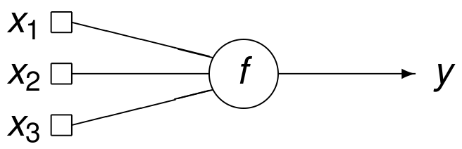
Fig. 69 A schematic of a neuron with three inputs and one output.

Two concrete examples of the function f are

\[y = \tanh \left( \sum_{i=1}^n w_i x_i + w_{n+1} \right)\]

and

\[y = \exp \left( - \sum_{i=1}^n (x_i - w_i)^2 \Big/ (2 w^2_{n+1}) \right).\]

Definition of a neural network.

A neural network is the composition of the nonlinear functions of two or more neurons.

An example of a neural network is defined as

\[y = g({\bf x}, {\bf w}) = \sum_{i=1}^{N_c} \left( w_{N_c+1, i} \tanh \left( \sum_{j=1}^n w_{i,j} x_j + w_{i,n+1} \right) \right) + w_{N_c+1, n+1}\]

where

• \(\bf x\) is the input vector, of \(n\) inputs, or variables, and

• \(\bf w\) is the vector of \((n+1)N_c + N_c + 1\) parameters, or weights.

The network shown in Fig. 70

• has three inputs with one bias \(x_0 = 1\),

• has three hidden neurons, and

• one linear output neuron.

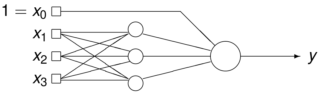
Fig. 70 An example of a neural network.

Definition of training of a neural network.

The training of a neural network is the algorithmic procedure

• whereby the parameters of the neurons of the network are estimated,

• in order for the network to fulfill the tasks it is assigned to do.

Two categories of training are considered:

1. supervised training: we know the nonlinear function analytically, or numerical values of the function are known.

2. unsupervised training: no supervision.

The training of a neural network can be viewed as a function approximation problem, where we keep in mind the following two properties.

1. Nonlinear in their parameters, neural networks are universal approximators.

Proposition of the existence proof.

Any bounded, sufficiently regular function can be approximated uniformly, with arbitrary accuracy in a finite region of variable space, by a neural network with a single layer of hidden neurons, having the same activation function, and a linear output neuron.

2. The most parsimonious model has the smallest number of parameters.

An Artificial Neural Network

The training of a neural network will be illustrated via the processing of a collection of labeled points, shown in Fig. 71. We could interpret the labels of the points as the outcome of a probe for oil. With the neural network we would like to predict the size of the oil field, or the location for where to drill next.

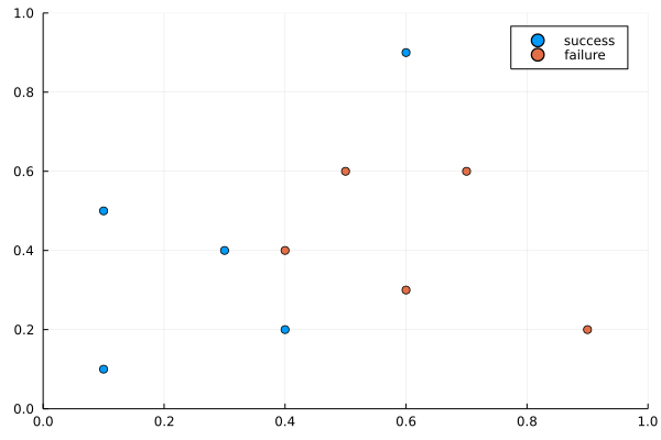
Fig. 71 A collection of labeled points.

The coordinates of the points are given in two vectors:

x1 = [0.1,0.3,0.1,0.6,0.4,0.6,0.5,0.9,0.4,0.7]
x2 = [0.1,0.4,0.5,0.9,0.2,0.3,0.6,0.2,0.4,0.6]

and their labels are defined as

y = [ones(1,5) zeros(1,5); zeros(1,5) ones(1,5)]

2x10 Matrix{Float64}:
 1.0  1.0  1.0  1.0  1.0  0.0  0.0  0.0  0.0  0.0
 0.0  0.0  0.0  0.0  0.0  1.0  1.0  1.0  1.0  1.0

The problem can then be formulated as follows. Find a function \(F\), so \(y = F(z_1, z_2)\), for a point \((z_1, z_2)\). To solve this problem, we use sigmoid functions. The sigmoid function is

\[\sigma(x) = \frac{1}{1 + e^{-x}}\]

and it can be viewed as a smoothed version of a step function, shown in Fig. 72.

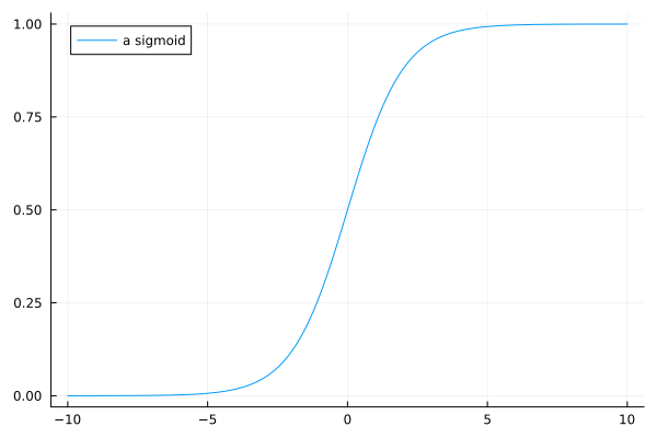
Fig. 72 The sigmoid function \(\sigma(x) = 1/(1 + e^{-x})\).

A scaled and shifted sigmoid function \(\sigma(3(x-5))\) is shown in Fig. 73.

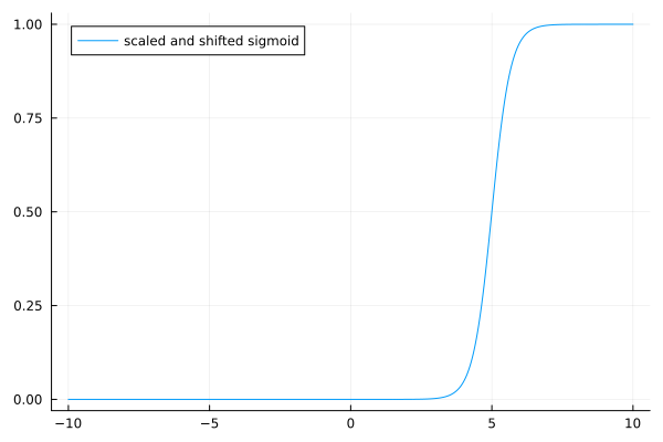
Fig. 73 The scaled and shifted sigmoid \(\sigma(3(x-5))\).

A Julia function for \(\sigma(W x + b)\) is listed below:

"""
    function activate(x,W,b)

evaluates the sigmoid function at x,
with weight matrix W and bias vector b.
"""
function activate(x,W,b)
    dim = size(W,1)
    y = zeros(dim)
    argexp = -(W*x + b)
    for i=1:dim
        y[i] = 1.0/(1.0 + exp(argexp[i]))
    end
    return y
end

The dimensions of the variables x, W, and b are as follows: if \(\mbox{x} \in {\mathbb R}^n\), \(\mbox{W} \in {\mathbb R}^{m \times n}\), \(\mbox{b} \in {\mathbb R}^m\), then \(\mbox{y} \in {\mathbb R}^m\).

The Julia function implements a neural network as

function F(x, W2, W3, W4, b2, b3, b4)
    a2 = activate(x, W2, b2)
    a3 = activate(a2, W3, b3)
    a4 = activate(a3, W4, b4)
    return a4
end

and it computes

\[\begin{split}\begin{array}{rcl} a_2 & = & \sigma(\mbox{W2*} \mbox{x} + \mbox{b2}) \\ a_3 & = & \sigma(\mbox{W3*} a_2 + \mbox{b3}) \\ a_4 & = & \sigma(\mbox{W4*} a_3 + \mbox{b4}) \end{array}\end{split}\]

which can be represented as in Fig. 74.

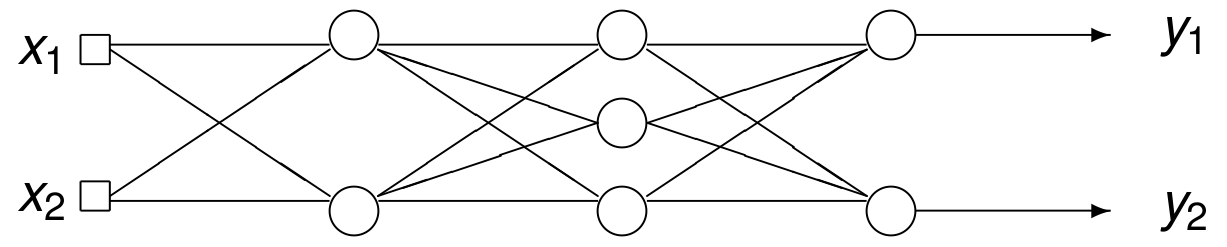
Fig. 74 The layers in an artificial neural network.

The weights and bias vectors in this neural network define the function

\[F(x) = \sigma(~\!\mbox{W4 }\! \sigma(~\!\mbox{W3 }\! \sigma(~\!\mbox{W2 }\!\mbox{x} + \mbox{b2}) + \mbox{b3}) + \mbox{b4})\]

which produces labels for each point. The cost function is

\[\mbox{Cost}\left( \vphantom{\frac{1}{2}} \mbox{W2}, \mbox{W3}, \mbox{W4}, \mbox{b2}, \mbox{b3}, \mbox{b4} \right) = \frac{1}{10} \sum_{i=1}^{10} \frac{1}{2} \Big\| y\left(x_1^{(i)}, x_2^{(i)}\right) - F\left(x_1^{(i)}, x_2^{(i)}\right) \Big\|_2^2.\]

The first exercise asks to count the number of parameters in the neural network defined by the function \(F\).

The problem of constructing the neural network is now reduced to minimizing the cost function. For this optimization problem, we consider Taylor series and the gradient vector. Assume the current vector is \(p = (p_1, p_2, \ldots, p_N)\).

Consider the Taylor series of the cost function at \(p\):

\[\mbox{Cost}(p + \Delta p) = \mbox{Cost}(p) + \sum_{i=1}^N \left( \frac{\partial \mbox{Cost}}{\partial p_i}(p) \right) \Delta p_i + O(\| \Delta p \|^2).\]

Denoting the gradient vector

\[\nabla \mbox{Cost}(p) = \left( \frac{\partial \mbox{Cost}}{\partial p_1}(p) , \frac{\partial \mbox{Cost}}{\partial p_2}(p) , \ldots , \frac{\partial \mbox{Cost}}{\partial p_N}(p) \right)\]

and ignoring the \(O(\| \Delta p \|^2)\) term:

\[\mbox{Cost}(p + \Delta p) \approx \mbox{Cost}(p) + \left( \vphantom{\frac{1}{2}} \nabla \mbox{Cost}(p) \right)^T \Delta p.\]

Minimizing the cost function is the objective. In an iterative method we replace \(p\) by \(p + \Delta p\), choosing \(\Delta p\) that makes \(\displaystyle \left( \vphantom{\frac{1}{2}} \nabla \mbox{Cost}(p) \right)^T \Delta p\) as negative as possible. By application of the Cauchy-Schwartz inequality:

\[\left| \left( \vphantom{\frac{1}{2}} \nabla \mbox{Cost}(p) \right)^T \Delta p ~ \right| \leq \left\| \vphantom{\frac{1}{2}} \nabla \mbox{Cost}(p) \right\|_2 \| \Delta p \|_2.\]

Therefore, choose \(\Delta p\) in the direction of \(-\nabla \mbox{Cost}(p)\). Update \(p\) as \(p = p - \eta \nabla \mbox{Cost}(p)\), where the step size \(\eta\) is called the learning rate. As we have a large number of parameters and many training points, the computation of the gradient vector at each step is too costly. Instead, take one single, randomly chosen training point, and evaluate the gradient at that point. This gives rise to the stochastic gradient method.

To run the stochastic gradient method, we need to evaluate the derivatives efficiently. Let \(a^{(1)} = x\), then the network returns \(a^{(L)}\), where

\[\begin{split}\begin{array}{rcl} z^{(\ell)} & = & W^{(\ell)} a^{(\ell-1)} + b^{(\ell)} \\ a^{(\ell)} & = & {\displaystyle \sigma \left( z^{(\ell)} \right)}, \quad \mbox{for} ~\ell = 2, 3, \ldots, L. \end{array}\end{split}\]

Let \(C\) be the cost, define \(\displaystyle \delta_j^{(\ell)} = \frac{\partial C}{\partial z_j^{(\ell)}}\) as the error of neuron \(j\) at layer \(\ell\).

By the chain rule, we have (with \(\circ\) as the componentwise product):

\[\begin{split}\begin{array}{rcl} \delta^{(L)} & = & \sigma'(z^{(L)}) \circ (a^{(L)} - y) \\ \delta^{(\ell)} & = & \sigma'(z^{(\ell)}) \circ (W^{(\ell+1)})^T \delta^{(\ell+1)} \\ {\displaystyle \frac{\partial C}{\partial b_j^{(\ell)}}} & = & \delta_j^{(\ell)} \quad \mbox{and} \quad {\displaystyle \frac{\partial C}{\partial w_{j,k}^{(\ell)}}} ~~ = ~~ \delta_j^{(\ell)} a^{(\ell - 1)}. \end{array}\end{split}\]

Sigmoids have convenient derivatives: \(\sigma'(x) = \sigma(x) ( 1 - \sigma(x))\).

The formulas lead to the following algorithm:

1. The forward pass evaluates \(a^{(1)}, z^{(2)}, a^{(2)}, z^{(3)}, \ldots, a^{(L)}\).

2. The backward pass evaluates \(\delta^{(L)}, \delta^{(L-1)}, \ldots, \delta^{(2)}\).

This way of computing gradients is back propagation.

The Julia code to train the network is listed below:

eta = 0.05
Niter = 1000000
for counter = 1:Niter
    k = rand((1:10), 1)[1]
    x = [x1[k], x2[k]]
    # Forward pass
    a2 = activate(x,W2,b2)
    a3 = activate(a2,W3,b3)
    a4 = activate(a3,W4,b4)
    # Backward pass
    delta4 = a4.*(ones(length(a4))-a4).*(a4-y[:,k])
    delta3 = a3.*(ones(length(a3))-a3).*(W4'*delta4)
    delta2 = a2.*(ones(length(a2))-a2).*(W3'*delta3)
    # Gradient step
    W2 = W2 - eta*delta2*x'
    W3 = W3 - eta*delta3*a2'
    W4 = W4 - eta*delta4*a3'
    b2 = b2 - eta*delta2
    b3 = b3 - eta*delta3
    b4 = b4 - eta*delta4
end

The output of

Z = [[x1[k], x2[k]] for k=1:10]
Y = [F(z, W2, W3, W4, b2, b3, b4) for z in Z]

is

10-element Vector{Vector{Float64}}:
 [0.9914991960849379, 0.008456961045118156]
 [0.9938902272050594, 0.006075750247468293]
 [0.998360435186392, 0.001628134278139295]
 [0.9865419031464729, 0.01338759273828821]
 [0.9737963089611226, 0.02615530711128986]
 [0.013028283269915059, 0.9869736384774328]
 [0.016354675508034607, 0.9837066212812329]
 [0.0005627461156236613, 0.9994383300176262]
 [0.02106910309704885, 0.979014892476464]
 [0.0012977070814389772, 0.9987047112752311]

The result of evaluating \(F(x_1, x_2)\) over \([0,1] \times [0,1]\) is shown in Fig. 75.

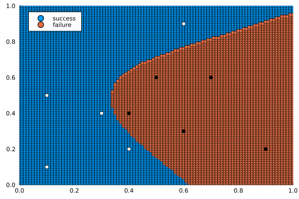
Fig. 75 Evaluating the trained neural network over \([0,1] \times [0,1]\).

The white and black dots in Fig. 75 are the ten given points.

Exercises

1. How many parameters are in the neural network defined by the function \(F(x)\)? Justify your answer.

2. Examine the computational cost to evaluate \(\nabla \mbox{Cost}(p)\) of our \(\displaystyle F(x) = \sigma(~\!\mbox{W4 }\! \sigma(~\!\mbox{W3 }\! \sigma(~\!\mbox{W2 }\!\mbox{x} + \mbox{b2}) + \mbox{b3}) + \mbox{b4})\).

3. How fast did the stochastic gradient method converge?

   1. Write a function to evaluate \(\mbox{Cost}(p)\).

   2. Call the function in the code to train the network, at each step, store the value of the cost function.

   3. Make a plot of the cost over all steps in the code.

Bibliography

1. Gerard Dreyfus: Neural Networks. Methodology and Applications. Springer-Verlag 2005.

2. Catherine F. Higham and Desmond J. Higham: Deep Learning: An Introduction for Applied Mathematicians. SIAM Review, Vol. 61, No. 4, pages 860-891, 2019.