Introduction to Deep Learning

We redo the example of an artificial neural network from the last lecture, but now with the Julia package Flux. As an illustration of a larger example, we consider the problem of recognizing handwritten numbers.

Getting Started with Flux

A workable definition of machine learning, also called learning from experience, is that a program learns from experience E with respect to some tasks T and performance measure P, if its performance at tasks in T, as measured by P improves with experience E.

Definition of a deep neural network.

A deep neural network is a neural network with multiple layers.

The illustration in Fig. 76 is taken from Deep Learning Notes using Julia with Flux, by Hugh Murrel and Nando de Freitas, available at <https://HughMurrel.github.io/DeepLearningNotes>, 2019.

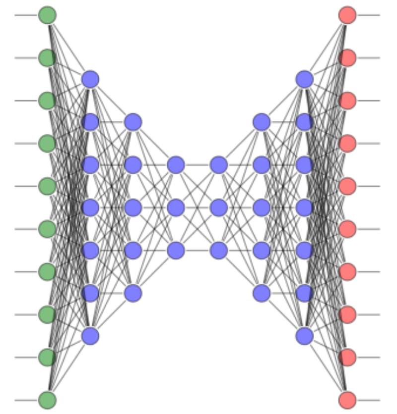
Fig. 76 A deep neural network.

Flux is a library for machine learning geared towards high-performance production pipelines, written entirely in Julia. Our first example comes from the quickstart documentation of Flux.

Let us go through an example, step-by-step:

1. define the task

2. get training data

3. define and initialize the model

4. define the loss function

5. set the optimizer

6. train the model

step 1: the task

Consider a weight matrix \(W_{\mbox{true}}\) and bias vector \(b_{\mbox{true}}\):

\[\begin{split}W_{\mbox{true}} = \left[ \begin{array}{ccccc} 1 & 2 & 3 & 4 & 5 \\ 5 & 4 & 3 & 2 & 1 \end{array} \right], \quad b_{\mbox{true}} = \left[ \begin{array}{c} -1 \\ -2 \end{array} \right].\end{split}\]

\(W_{\mbox{true}}\) and \(b_{\mbox{true}}\) are parameters in the function

\[F_{\mbox{true}}(x) = W_{\mbox{true}} x + b_{\mbox{true}}\]

which

• takes on input \(x\), a vector of five numbers, and

• return \(y = F(x)\), a vector of two numbers.

Then the task is to recover \(W_{\mbox{true}}\) and \(b_{\mbox{true}}\) from observed \((x_{\mbox{train}}, y_{\mbox{train}})\).

step 2: training data

Let \(N\) be the size of the training vectors \(x_{\mbox{train}}\) and \(y_{\mbox{train}}\). Then,

• the i-th vector of \(x_{\mbox{train}}\) is \(x_i\), and

• the i-th vector of \(y_{\mbox{train}}\) is \(y_i\),

with

\[\begin{split}x_i = \left[ \begin{array}{c} 5 + 5 u_{1,i} \\ 5 + 5 u_{2,i} \\ 5 + 5 u_{3,i} \\ 5 + 5 u_{4,i} \\ 5 + 5 u_{5,i} \end{array} \right], \quad z_i = F(x_i), \quad y_i = \left[ \begin{array}{c} z_{1,i} + 0.2 v_{1,i} \\ z_{2,i} + 0.2 v_{2,i} \end{array} \right],\end{split}\]

where \(i\) runs from 1 to \(N\), and

• \(u_{j,i}\) are chosen at random, uniformly from \([0,1]\).

• \(v_{j,i}\) are random, standard normally distributed numbers.

step 3: defining and initializing the model

The model is

\[M(x) = W x + b, \quad W \in {\mathbb R}^{2 \times 5}, \quad b \in {\mathbb R}^{2}.\]

We initialize \(M(x)\) with

1. a random 2-by-5 matrix for \(W\), and

2. a random 2-vector for \(b\).

step 4: the loss function

The performance is measured by a loss function:

\[\mbox{loss}(x, y) = \sum_{i=1}^2 \left( \vphantom{\frac{1}{2}} y_i - \widehat{y}_i \right)^2, \quad y = F(x), \quad {\widehat{y}} = M(x).\]

step 5: set an optimizer

We choose the classic gradient descent as the optimizer with learning rate \(\eta = 0.01\).

step 6: train the model

Flux.train!(loss, params(W, b), train_data, opt)

To train the model, the longer way is in the code below:

opt = Descent(0.01)
train_data = zip(x_train, y_train)
ps = Flux.params(W, b)
for (x, y) in train_data
    gs = gradient(ps) do
        loss(x,y)
    end
    Flux.Optimise.update!(opt, ps, gs)
end

The main benefit of this lower way to train the model is that we can monitor the progress of the loss function.

An Artificial Neural Network Revisited

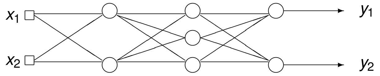
Fig. 77 The layers in an artificial neural network.

The artificial neural network of the last lecture is shown in Fig. 77. We will redo the training of this model with Flux. The weights and the bias vectors are

\[\mbox{W2} \in {\mathbb R}^{2 \times 2}, \mbox{W3} \in {\mathbb R}^{3 \times 2}, \mbox{W4} \in {\mathbb R}^{2 \times 3}, \mbox{b2} \in {\mathbb R}^{2}, \mbox{b3} \in {\mathbb R}^{3}, \mbox{b4} \in {\mathbb R}^{2}.\]

With Flux.jl, we define the model as

L2 = Dense(W2, b2, sigmoid)
L3 = Dense(W3, b3, sigmoid)
L4 = Dense(W4, b4, sigmoid)
M = Chain(L2, L3, L4)

In the code above, L2 = Dense(W2, b2, sigmoid) makes one layer with weights W2, bias b2, and the sigmoid function. Multiple layers into one network are collected by M = Chain(L2, L3, L4). The output is

Chain(
  Dense(2 => 2, \sigma),   # 6 parameters
  Dense(2 => 3, \sigma),   # 9 parameters
  Dense(3 => 2, \sigma),   # 8 parameters
 )    # Total: 6 arrays, 23 parameters, 568 bytes.

Observe that this output solves the first exercise of the last lecture on the number of parameters in the model.

To train the network, we define next the loss function. The loss function is

\[\mbox{loss}\left( \vphantom{\frac{1}{2}} \mbox{W2}, \mbox{W3}, \mbox{W4}, \mbox{b2}, \mbox{b3}, \mbox{b4} \right) = \frac{1}{10} \sum_{i=1}^{10} \frac{1}{2} \Big\| y\left(x_1^{(i)}, x_2^{(i)}\right) - M\left(x_1^{(i)}, x_2^{(i)}\right) \Big\|_2^2,\]

where \(M\) is the model, defined in the code below:

function loss(x, y)
    result = 0.0
    for i=1:10
        point = [x1[i]; x2[i]]
        yy = M(point)
        result = result + 0.5*((yy[1] - ylabels[1,i])^2
                             + (yy[2] - ylabels[2,i])^2)
    end
    return result/10.0
end

Defining the training data and the optimizer, we take one million data points:

N = 1_000_000
xtrain = [randn(2) for _ in 1:N];
ytrain = [randn(2) for _ in 1:N];

We define the optimizer and parameters:

train_data = zip(xtrain, ytrain)
opt = Descent(0.01)
ps = Flux.params(M)

Then the training of the model, happens via

Flux.train!(loss, ps, train_data, opt)

Evaluating \(F(x_1, x_2)\) over \([0,1] \times [0,1]\) produces similar plots as in the previous lecture.

Recognizing Handwritten Numbers

So far, our neural networks have been small. In this section we consider a larger problem. The MNIST database of handwritten digits is a classic image classification dataset with 70,000 images, available at <http://yann.lecun.com/exdb/mnist>. The data is described in the paper Gradient-based learning applied to document recognition by Y. LeCun, L. Bottou, Y. Bengio, and P. Haffner, published in the Proceedings of the IEEE, November 1998

In Julia, we access this data set as follows:

julia> using MLDatasets: MNIST

julia> MNIST.download()

The preparation of this lecture benefited from the post at <https://machinelearninggeek.com/mnist-with-julia>.

The first five images are shown in Fig. 78 and labeled as 5, 0, 4, 1, and 9.

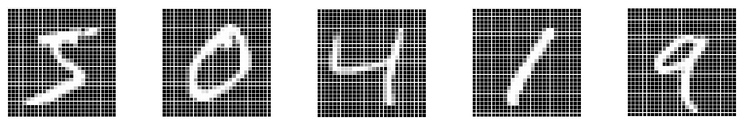
Fig. 78 The first five images in the MNIST data base.

• The i-th image is available as MNIST(split=:train).features[:,:,i}].

• Its corresponding label is in MNIST(split:=train).targets[\mbox{i}].

The training of the network will be described in a step-by-step fashion.

step 1: representing the labels as vectors

Consider the statements:

using Flux: onehotbatch

labels = onehotbatch(MNIST(split=:train).targets, 0:9)

With onehotbatch, each trainlabel is converted to a vector, As MNIST(split=:train).targets[i] returns an integer in the range from 0 to 9, the vector that corresponds to the label will have length 10. The vector will be zero, except for a one at the entry the corresponds to the value of the label. For example, the number 5 corresponds to the vector

\[[0, 0, 0, 0, 0, 1, 0, 0, 0, 0]^T.\]

step 2: representing the images as vectors

The images are 28-by-28 matrices of UInt8 types. The code below takes the first 100 images, reshapes the matrix into a vector and converts the numbers.

NBR = 100
images = Matrix{Float32}(zeros(28*28, NBR))
for i=1:size(images,2)
    image = MNIST(split=:train).features[:,:,i]
    imagereshaped = reshape(image,:)
    imagenumbers = [Float32(x) for x in imagereshaped]
    for j=1:size(images,1)
        images[j, i] = imagenumbers[j]
    end
end

step 3: defining the model

We define the model as follows:

using Flux

model = Chain(Dense(28*28, 40, relu), Dense(40, 10), softmax)

where

• relu stands for rectified linear output, and

• softmax formulates a logistic regression.

The output is of the Chain statement is

Chain(
  Dense(784 => 40, relu), # 31_400 parameters
  Dense(40 => 10),        # 410 parameters
  NNlib.softmax,
)  # Total: 4 arrays, 31_810 parameters, 124.508 KiB.

Observe the large number of parameters. To test if the definition is valid, we evaluate at the 10-th image: model(images[:,10]).

step 4: the loss function

In classifications with multiple classes, where the labels are given in a one-hot format, we use:

using Flux: crossentropy

loss(X, y) = crossentropy(model(X), y)

step 5: select the optimizer

The optimizer is set to one of the gradient descent methods:

opt = Adam()

Adam is a variation of Adaptive Gradient Descent where the components of the gradient are weighted.

step 6: training the model

To monitor the progress during the training, we define a callback function:

progress = () -> @show(loss(images, labels[:,1:NBR]))

Then the training happens as follows:

using Flux: throttle
for epoch in 1:100
    Flux.train!(loss, Flux.params(model),
        [(images,labels[:,1:NBR])], opt,
        cb = throttle(progress, 10))

The loss is reported every 10 seconds. One epoch loops over the data only once. In the training, we limited the number of epochs to 100.

To verify the model, we evaluate an image in the model, and then check for the index of the largest value:

M1 = model(images[:,1])
println("output of the model :\n", M1)
println("the number is ", argmax(M1)-1)

The first five image are classified correctly.

To check a random image from the training data:

idx = rand((1:NBR),1)
Midx = model(images[:,idx[1]])
println("output of the model :\n", Midx)
println("the number is ", argmax(Midx)-1)
println("label : ", MNIST(split=:train).targets[idx])

Proposal of a Project Topic

1. Machine learning with Flux.

   One software that learns from experience is Flux.

   1. Read the software documentation.

   2. Describe how it fits in the computational ecosystem of Julia.

   3. Illustrate the capabilities by a good use case.

      Do not use MNIST, but a similar good data set.

   What is scientific machine learning?

Exercises

1. For the first example with Flux, make a plot of the loss function for all \(N\) steps. Does \(N\) really have to be 10,000 for sufficient accuracy?

2. In our artificial neural network, do we really need one million data points? Plot the evolution of the loss function for all steps.

3. In our artificial neural network, what if we use rand instead of randn in the definition of the xtrain and ytrain vectors?

4. After training the neural network on the MNIST data, verify a random image that is not in the training data.

Bibliography

1. Catherine F. Higham and Desmond J. Higham: Deep Learning: An Introduction for Applied Mathematicians. SIAM Review, Vol. 61, No. 4, pages 860-891, 2019.

2. Michael Innes, Elliot Saba, Keno Fischer, Dhairya Gandhi, Marco Concetto Rudilosso, Neethu Mariya Joy, Tejan Karmali, Avik Pal, and Viral Shah: Fashionable Modelling with Flux, <https://arxiv.org/abs/1811.01457>, 2018.

3. Y. LeCun, L. Bottou, Y. Bengio, and P. Haffner: Gradient-based learning applied to document recognition. Proceedings of the IEEE, 86(11):2278-2324, November 1998 <http://yann.lecun.com/exdb/mnist>.

3. Hugh Murrel and Nando de Freitas: Deep Learning Notes using Julia with Flux, <https://HughMurrel.github.io/DeepLearningNotes>, 2019.