Face Recognition and Ranking Data
This lecture covers two topics in data science.
Face Recognition
Face recognition is challenging because of the position of the head, lightning conditions, and moods and expressions. Many automated systems have been developed. A linear algebra approach is based on eigenfaces, a method proposed by Sirovich and Kirby, 1987.
The input is a p-by-q grayscale image. The resolution of an image is \(m = p \times q\). All images of the same resolution live in an m-dimensional space. The subspace of all facial images} has a low dimension, independent of the resolution.
This result is described in the paper on Singular Value Decomposition, Eigenfaces, and 3D Reconstructions by Neil Muller, Lourenco Magaia, B. M. Herbst, SIAM Review, Vol. 46, No. 3, pages 518-545, 2004.
The singular value decomposition of a p-by-q matrix \(A\) is
where \(U\) and \(V\) are orthogonal: \(U^{-1} = U^T\), \(V^{-1} = V^T\), and \(\Sigma\) is a diagonal matrix, with on its diagonal
are the singular values of the matrix \(A\).
If \(\mbox{rank}(A) = r\), then \(\sigma_i = 0\) for all \(i > r\). Ignoring the smallest singular values leads to a dimension reduction.
The geometric interpretation of the singular value decomposition is illustrated in Fig. 79.
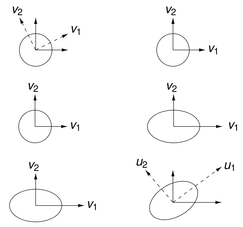
Fig. 79 Computing \(U \Sigma V^T\) corresponds to rotating a circle, stretching the circle into an ellipse, and then rotating the ellipse.
The singular values and vectors relate to the eigenvalues and eigenvectors as follows. By the singular value decomposition of \(A\):
This implies
The largest singular value measures the magnitude of \(A\):
In machine learning, the eigenfaces method is known as the Principal Component Analysis (PCA). The procedure by Neil Muller et al. is summarized below:
The XM2VTS Face Database of the University of Surrey at <http://www.ee.surrey.ac.uk/Research/VSSP/xm2vtsdb> consists of many RGB color images against a blue background.
The background is removed by color separation.
Averaging RGB values, the images were converted to grayscale.
A training set has 600 images, 3 of each, for 200 individuals.
If the training set is representative, then all facial images would be in a 150-dimensional subspace.
What is the typical range of measurements of a face? Consider \(n\) measurements \((x_i, y_i)\) for \(i=1,2,\ldots,n\), where
\(x_i\) is the width, measured ear-to-ear, and
\(y_i\) is the height, measured from chin to between the eyes.
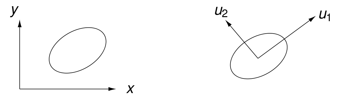
Fig. 80 A coordinate change defined by the axes of an ellipse.
Assume all \(n\) measurements lie within an ellipse as shown in Fig. 80. Then, the coordinate change to \(u_1\) and \(u_2\) as in Fig. 80 is computed via a singular value computations on a shifted matrix.
To find then the typical range of width and height of a face:
Compute the mean \((\overline{x}, \overline{y})\) of all \(n\) observations.
Subtract \(\overline{x}\) from all \(x_i\) and subtract \(\overline{y}\) from all \(y_i\).
Divide the \(n\) shifted observations by \(\sqrt{n}\).
Apply the singular value decomposition on the matrix \(A\), which has in its columns the shifted observations.
The first two columns of \(U\) give the directions of maximum variations and the two largest singular values are the magnitudes of the standard deviations in those two directions. With the mean and standard deviation of the measurements, we can define a normal distribution. The farther observations fall outside the normal ellipse, the less likely the measurements represent a face.
Stacking the columns of the images into one vector, we obtain a matrix \(F = [f_j \mbox{ is stacked image for } j=1,2,\ldots,n]\).
Compute the mean \(\displaystyle \mu = \frac{1}{n} \sum_{j=1}^n f_j\).
Shift the data \(a_j = x_j - \mu\), \(j=1,2,\ldots,n\).
Define the matrix
\[A = \frac{1}{\sqrt{n}} \left[ \vphantom{\frac{1}{2}} ~~ x_1 ~~ x_2 ~~ \cdots ~~ x_n ~~ \right].\]Compute the singular value decomposition \(A = U \Sigma V^T\).
The columns of \(U\) are the eigenvectors of \(A A^T\) (the covariance matrix). Those columns of \(U\) are the eigenfaces of F
The mean of the training set is \(\mu\). The matrix \(U\) is orthogonal. Use the first \(\nu\) eigenfaces:
For any image \(f\) (as a stacked vector), compute its projection
with is the eigenface representation of f. Then the eigenface reconstruction of f is \(\widetilde{f} = U_\nu y + \mu\). Comparing the reconstructed faces to the given ones in the training set leads to the finding of the best value for \(\nu\).
The three steps in the Principal Component Analysis are listed below:
Three steps:
Standardize the data, via the formula
\[z = \frac{x - \mbox{mean}}{\mbox{standard deviation}},\]applied to each number \(x\) in the input.
Setup the covariance matrix \(C\). For each pair \((z_i, z_j)\),
\[{\rm cov}(z_i, z_j) \mbox{ is the } (i,j)\mbox{-th element of the matrix.}\]The matrix \(C\) is symmetric and positive definite.
Compute the eigenvectors and eigenvalues of \(C\).
Sort the eigenvectors in increasing magnitude of the eigenvalues.
Then the feature vector consist of the first \(p\) eigenvectors.
Ranking Data
To build a search engine, the following problem must be solved:
This is an engineering challenge, as the search engine must answer tens of millions of queries each day. Google is designed to be a scalable search engine.
The crawlable web is a graph of pages (nodes) and links (edges).
Every page has forward links (outedges) and backlinks (inedges).
Highly linked pages are more important than pages with few links.
The rank of page \(u\) is \(\displaystyle R(u) = c \sum_{v \in B_u} \frac{R(v)}{N_v}\).
\(N_u\) is the number of pages the page \(u\) points to.
\(B_u\) is the number of pages that point to \(u\).
\(c < 1\) because many pages do not point to any other pages.
Let \(A\) be a square matrix indexed by web pages.
\(A_{u, v} = 1/N_u\), if there is an edge from \(u\) to \(v\),
\(A_{u, v} = 0\), otherwise.
Consider the vector \(R = [R(u) \mbox{ for all pages } u]\), then:
so \(R\) is an eigenvector of \(A\) with eigenvalue \(1/c\).
For an example on the evaluation of \(\displaystyle R(u) = c \sum_{v \in B_u} \frac{R(v)}{N_v}\) consider the simple 4-page web as shown in Fig. 81.
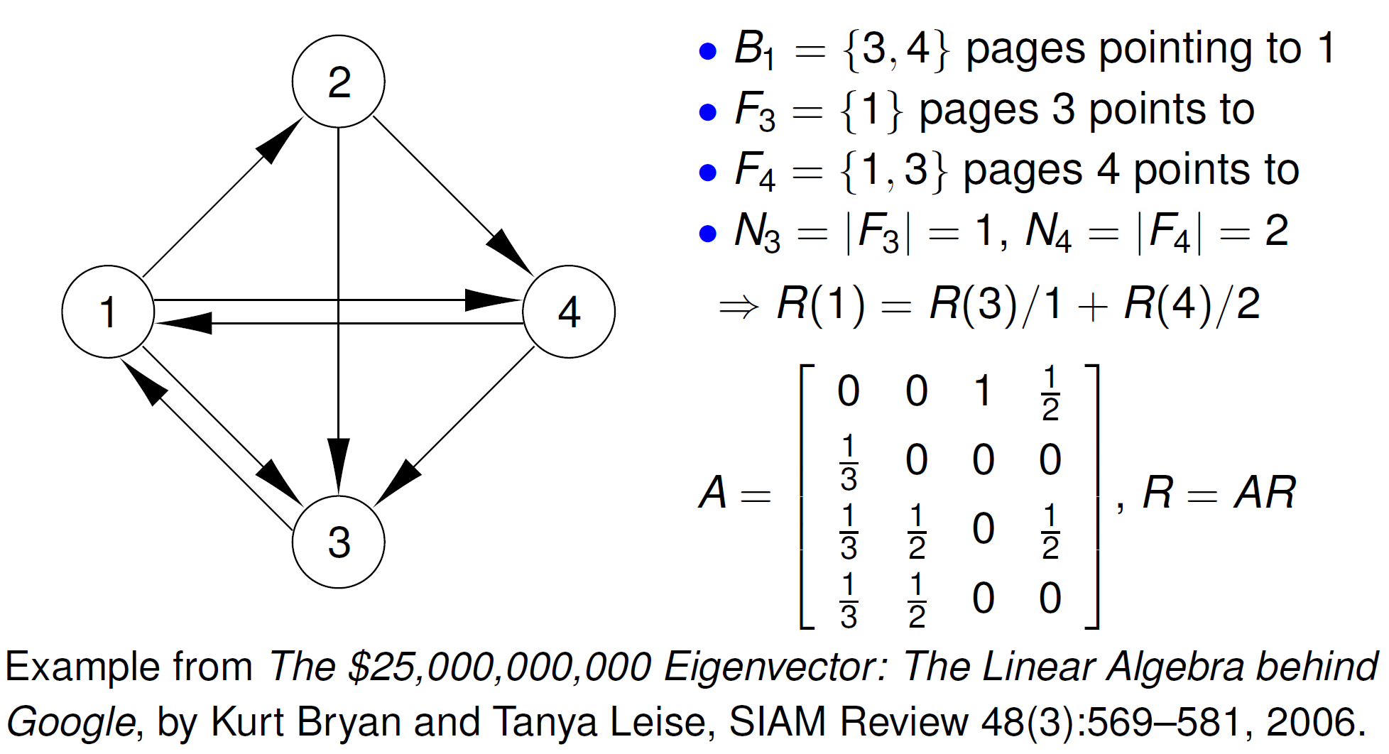
Fig. 81 Setting up the matrix for a 4-page web defined by the directed graph.
For the example in Fig. 81, which of the 4 pages scores highest? Consider the computational session below.
julia> A = [0 0 1 1/2; 1/3 0 0 0; 1/3 1/2 0 1/2; 1/3 1/2 0 0]
4x4 Matrix{Float64}:
 0.0       0.0  1.0  0.5
 0.333333  0.0  0.0  0.0
 0.333333  0.5  0.0  0.5
 0.333333  0.5  0.0  0.0

julia> using LinearAlgebra

julia> L, V = eigen(A);

julia> L
4-element Vector{ComplexF64}:
 -0.36062333350611053 - 0.4109755454950538im
 -0.36062333350611053 + 0.4109755454950538im
   -0.278753332987779 + 0.0im
    1.000000000000002 + 0.0im

julia> V[:,4]
4-element Vector{ComplexF64}:
  0.7210101217513317 + 0.0im
 0.24033670725044398 + 0.0im
  0.5407575913134985 + 0.0im
 0.36050506087566603 + 0.0im
As the first component of the dominant eigenvector is highest, we conclude that page 1 scores highest. Observe that the largest eigenvalue equals one, as we have taken the constant \(c\) as one.
The problem with the simplified PageRank is a rank sink caused by two pages pointing to each other but to no other page, and one third page pointing to one of those two pages. Therefore, the simplified PageRank is modified as follows:
The 1-norm is \(\| R \|_1 = |R_1| + |R_2| + \cdots + |R_n|\), \(n\) is the length of \(R\). In matrix notation: \(R' = c (A~\!R' + E)\).
To compute the PageRank, we introduce the random surfer model. The PageRank can be derived from random walks in graphs. If a surfer ever gets in a small loop of web pages, then the surfer will most likely jump out of the loop. The likelihood of a surfer jumping to a random page is modeled by \(E\) in
The algorithm to compute the PageRank is outlined below:
Initialize \(R_0\) to some random vector.
do
\(R_{i+1} = A~\!R_i\)
\(d = \| R_i \|_1 - \| R_{i+1} \|_1\)
\(R_{i+1} = R_i + d~\!E\)
\(\delta = \| R_{i+1} - R_i \|_1\)
while \(\delta > \epsilon\).
We recognize a variant of the power method to compute the eigenvector associated with the dominant eigenvalue.
Let \(P = [p_{i,j}]\) a square matrix, with indices \(i\) and \(j\) running over all web pages, \(p_{i,j}\) is the probability of moving from page \(j\) to page \(i\). Because the \(p_{i,j}\)’s are probabilities, the sum of all elements in the j-th column of \(P\) equals one. The matrix \(P\) is called a stochastic matrix. We can look to the equation \(x = c~\!P x\), which corresponds to the simplified PageRank definition.
To model the likelihood that a surfer jumps out of a loop:
With probability \(\alpha\), in the next move the surfer follows one outedge at page \(j\).
With probability \(1 - \alpha\), the surfer teleports to any other page according to the distribution vector \(v\).
Then we arrive at the equation
The constant \(\alpha\) is called the teleportation parameter.
The search engine problem is reduced to the PageRank problem.
This reduces the PageRank problem to solving a linear system. For the relation with eigenvectors, consider summing up the entries in the column stochastic vector \(v\):
Then we rewrite \((I - \alpha P) x = (1 - \alpha) v\) as
In the rewrite we applied \(e^T x = 1\), as the PageRank vector is a column stochastic vector.
The mathematics of PageRank apply to any graph or network and the ideas occur in a wide range of applications:
GeneRank and ProteinRank in bioinformatics
IsoRank in ranking graph isomorphisms
PageRank of the Linux kernel
Roads and urban spaces
PageRank of winner networks in sports
BookRank in literature, recommender systems
AuthorRank in the graph of coauthors
Paper and citation networks
proposal for a project topic
Read the paper and consider the software:
Florian Schroff, Dmitry Kalenichenko, and James Philbin:
FaceNet: A Unified Embedding for Face Recognition and Clustering. <https://arxiv.org/abs/1503.03832>
OpenFace: free and open source face recognition with deep neural networks. <https://cmusatyalab.github.io/openface/>
Do the following:
Read the paper and install the software.
Experiment with many pictures of the same two people.
Train the neural network to recognize the faces on the first half of the pictures. Test the neural network on the second half.
What is the success rate? Can you improve the selection of the pictures? What if passport style pictures are used?
Exercises
Verify that \(A = U \Sigma V^T\) implies \(A^T A V = V \Sigma^T \Sigma\) and \(A A^T U = U \Sigma \Sigma^T\).
In the algorithm to compute the PageRank, what about the growth of \(A~\!R_i\)? Why does the algorithm above not divide \(R\) by its largest component?
For the matrix \(A\) in the 4-page web example in Fig. 81 consider the linear system
\[(I - \alpha A){\bf x} = (1 - \alpha) {\bf v},\]with \(\alpha = 0.15\) and \(v_i = 1/4\), \(i=1,2,3,4\). Do the following:
Solve the linear system. Is the solution a column stochastic vector?
Compare the new rankings with the ones from before. Does page 1 still score highest?
Bibliography
S. Brin and L. Page: The anatomy of large-scale hypertextual web search engine. Computer Networks and ISDN systems 30, pages 107-117, 1998.
Kurt Bryan and Tanya Leise: The $25,000,000,000 Eigenvector: The Linear Algebra behind Google. SIAM Review, vol. 48, no. 3, pages 569-581, 2006.
David F. Gleich: PageRank Beyond the Web. SIAM Review, vol. 57, no. 3, pages 321-363, 2015.
Neil Muller, Lourenco Magaia, B. M. Herbst: Singular Value Decomposition, Eigenfaces, and 3D Reconstructions. SIAM Review, Vol. 46, No. 3, pages 518-545, 2004.
L. Page, S. Brin, R. Motwani, T. Winograd: The PageRank Citation Ranking: Bringing Order to the Web. Technical Report. Stanford InfoLab.