Laplace Transforms, Signals and Plants

With Laplace transforms, differential equations become algebraic equations.

The Frequency Domain

The Laplace transform takes a signal from the time domain, in \(t\), to the frequency domain, using \(s\) as the symbol in the transform.

Definition of the Laplace transform.

Given an integrable function \(f(t)\) in time \(t\), the Laplace transform of \(f(t)\) is

\[{\cal L}\{ f \} = \int_0^\infty f(t) e^{-s t} dt = F(s).\]

Because the integral operator is a linear operator, the Laplace transform is linear. In particular,

• Let \(f(t)\) and \(g(t)\) be two integrable functions.

• Let \(a\) and \(b\) be two coefficients, independent of \(t\).

Then

\[{\cal L}\{a f(t)+ b g(t)\} = a F(s) + b G(s),\]

where

• \(F(s)\) is the Laplace transform of \(f(t)\), and

• \(G(s)\) is the Laplace transform of \(g(t)\).

Another set of properties involves delay and exponentials. For some constant coefficient \(a\), we have:

• \(f(t - a)\) has Laplace transform \(e^{-as} F(s)\),

• \(e^{-at} f(t)\) has Laplace transform \(F(s+a)\),

• \(f(a t)\) has Laplace transform \(F(s/a)/a\).

What is s? Consider the Laplace transform of \(f(t) = 1\):

\[\begin{split}\begin{array}{rcl} {\displaystyle \int_0^\infty 1 e^{-s t} dt} & = & {\displaystyle \int_0^\infty \frac{-1}{s} e^{(-s t)} d(-st) } \\ & = & {\displaystyle \left. - \frac{e^{-s t}}{s} \right]_0^\infty} ~ = ~ 0 - \left( -\frac{1}{s} \right) = \frac{1}{s}. \end{array}\end{split}\]

This leads to

\[s \int_0^\infty 1 e^{-s t} dt = 1 \quad \mbox{or} \quad s {\cal L}\{ 1 \} = 1.\]

Multiplying with \(s\) can be called a generalized differentiation.

the Laplace transform of the derivative

\[{\cal L}\left\{ \frac{d}{d~\!t} f(t) \right\} = s F(s) - f(0), \quad F(s) = {\cal L}\{ f \}\]

Apply integration by parts: \(\displaystyle \int u dv = uv - \int v du\).

\[\begin{split}\begin{array}{rcl} {\displaystyle {\cal L}\left\{ \frac{d}{d~\!t} f(t) \right\}} & = & {\displaystyle \int_0^\infty e^{-st} \frac{d}{d~\!t} f(t) ~=~ \left. e^{-st} f(t) \vphantom{\frac{1}{2}} \right]_0^\infty - \int_0^\infty f(t) \frac{d}{d~\!t} e^{-st}} \\ & = & {\displaystyle 0 - f(0) - \int_0^\infty f(t) (-s) e^{-st} dt} \\ & = & -f(0) + s F(s) \end{array}\end{split}\]

Applying the property of the Laplace transform repeatedly, we arrive at the following:

the Laplace transform of the \(n\)-th derivative

For \(n>0\):

\[{\cal L}\left\{ \frac{d^n}{d~\!t^n} f(t) \right\} = s^n F(s) - s^{n-1} f(0) - s^{n-2} f'(0) - \cdots - f^{(n-1)}(0),\]

where \(F(s) = {\cal L}\{ f \}\).

We next explore symbolic computing, and the Laplace transform in SymPy.jl. Consider:

@syms s, t
one = sympy.laplace_transform(1, t, s)

which returns (1/s, 0, True).

sympy.inverse_laplace_transform(one[1], s, t)

returns \(\theta(t)\), defined below:

Definition of the Heaviside function

The Heaviside function is the piecewise function

\[\begin{split}\theta(t) = \left\{ \begin{array}{lcl} 1 & \mbox{if} & t > 0, \\ 1/2 & \mbox{if} & t = 0, \\ 0 & \mbox{if} & t < 0. \end{array} \right.\end{split}\]

The Heaviside function can also be seen as a limit of a smoothed step function, as

\[\lim_{k \rightarrow \infty} \left( 1 + e^{-2 k x} \right)^{-1}\]

and shown in Fig. 99 for increasing values of \(k\).

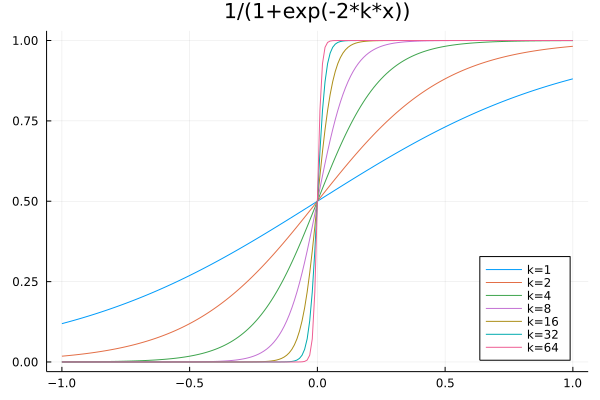
Fig. 99 The Heaviside function as the limit of a smoothed step function.

The sympy.inverse_laplace_transform used earlier is formally defined below.

Definition of the inverse Laplace transform

The inverse Laplace transform of \(F(s)\) is \(f\) with the property

\[{\cal L}\{ f \}(s) = F(s).\]

Observe the similarity between the Laplace transform of \(f(t)\) which is \(\displaystyle {\cal L}\{ f \} = \int_0^\infty f(t) e^{-s t} dt = F(s)\) with the continuous Fourier transforms:

Definition of the Fourier transform

The Fourier transform of \(f\) is

\[{\cal F} \{ f \} = \int_{-\infty}^{\infty} f(t) e^{-i \omega t} dt = F(i \omega).\]

Definition of the inverse Fourier transform

The inverse Fourier transform of \(F\) is

\[{\cal F}^{-1} \{ F \} = \frac{1}{2 \pi} \int_{-\infty}^{\infty} F(i \omega) e^{i \omega t} d \omega.\]

Operational Calculus

To solve an Ordinary Differential Equation (ODE), do:

1. Transform the ODE into the frequency domain.

2. Solve the algebraic equation in \(s\).

3. Transform the solution into the time domain.

Consider the following example:

\[\frac{d^2}{d~\!t^2} y(t) + 3 \frac{d}{d~\!t} y(t) + 2 y(t) = 1, \quad y(0) = 0, \quad y'(0) = 0.\]

1. Denoting \({\cal L}\{y\} = Y(s)\), the transformed equation is

   \[s^2 Y(s) + 3 s Y(s) + 2 Y(s) = \frac{1}{s}.\]

2. We solve the algebraic equation: \(s ( s+1 ) (s+2) Y(s) = 1\).

   \[Y(s) = \frac{1}{s (s+1) (s+2)} = \frac{1/2}{s} - \frac{1}{s+1} + \frac{1/2}{s+2}\]

3. Transformed back into the time domain, the solution is

   \[y(t) = \frac{1}{2} - e^{-t} + \frac{1}{2} e^{-2t}.\]

Consider the system of first order differential equations:

\[\begin{split}\left\{ \begin{array}{rcl} x' & = & -2x - 9y \\ y' & = & \hphantom{-2}x - 2y \end{array} \right. \quad x(0) = -1, \quad y(0) = 1.\end{split}\]

We apply the 3-step process:

1. Denoting \(X(s) = {\cal L}\{x\}\) and \(Y(s) = {\cal L}\{y\}\), the transformed system is

   \[\begin{split}\left\{ \begin{array}{rcl} sX + 1 & = & -2X - 9Y \\ sY - 1 & = & \hphantom{-2}X - 2Y \end{array} \right. \quad \mbox{or} \quad \left\{ \begin{array}{rcl} (s + 2)X + 9Y & = & - 1 \\ -X + (s+2)Y & = & 1 \end{array} \right.\end{split}\]

2. Use SymPy to solve the system.

   @syms X, Y
   eq1 = (s+2)*X + 9*Y + 1
   eq2 = -X + (s+2)*Y - 1
   sol = solve([eq1, eq2], [X, Y])
   

   has output

   Dict{Any, Any} with 2 entries:
    Y => (s + 1)/((s + 2)**2 + 9)
    X => -(s + 11)/(s**2 + 4*s + 13)
   

3. Transform the solution into the time domain.

   xt = sympy.inverse_laplace_transform(sol[X], s, t)
   

   returns \(-e^{-2t}(3 \sin(3t) + \cos(3t)) \theta(t)\) as \(x(t)\).

   yt = sympy.inverse_laplace_transform(sol[Y], s, t)
   

   returns \(-e^{-2t}(\sin(3t)/3 + \cos(3t)) \theta(t)\) as \(y(t)\).

Note: for \(t > 0\), we have \(\theta(t) = 1\) and we can drop \(\theta(t)\).

Generalizing the previous example to solving linear systems goes as follows. Let \(A\) be an n-by-n matrix and consider the system

\[\frac{d}{d~\!t} {\bf z}(t) = A {\bf z}, \quad {\bf z}(0) = {\bf z}_0.\]

1. Denoting \({\cal L}\{{\bf z}\} = {\bf Z}(s)\), the transformed equation is

   \[s {\bf Z}(s) - {\bf z}_0 = A.\]

2. The solution in the frequency domain is

   \[{\bf Z}(s) = (s I - A)^{-1} {\bf z}_0,\]

   where \(I\) is the identity matrix.

   If \(A\) has \(k\) distinct eigenvalues, then

   \[\det(s I - A) = \prod_{i=1}^k (s - \lambda_k)^{m_k},\]

   where \(m_k\) is the multiplicity of the k-th eigenvalue \(\lambda_k\).

   The matrix partial fraction expansion has then the form:

   \[(s I - A)^{-1} = \sum_{k=1}^r \sum_{j=1}^{m_k} \frac{v_{j,k}}{(s-\lambda_k)^j}.\]

3. Use the partial fraction expansion to transfer into the time domain.

Signals and Plants

We next define the convolution of continuous functions, make the connection between signals and ordinary differential equations.

Definition of convolutions of functions

Let \(f\) and \(g\) be functions of \(t\). The convolution \(f \star g\) of \(f\) and \(g\) is

\[f \star g = \int_0^t f(\tau) g(t - \tau) d \tau.\]

Recall the discrete convolution \(\displaystyle y_k = \sum_{i=0}^k h_i u_{k-i}\), where

• \(y_k\) is the k-th component of the output signal, \(y = h \star u\),

• \(h\) is the response of the unit impulse, and

• \(u\) is the input signal.

Applying the convolution to continous signals, for continuous input \(u(t)\), unit impulse response \(h(t)\), the output is then

\[y(t) = h(t) \star u(t)\]

is the continuous output of the filter. In the frequency domain:

\[Y(s) = H(s) U(s)\]

where the Laplace transforms are

\[U(s) = {\cal L}\{ u \}, \quad H(s) = {\cal L}\{ h \}, \quad \mbox{and} \quad Y(s) = {\cal L}\{ y \}.\]

Definition of a plant

A plant is a linear, time invariant, causal map, which maps signals into signals.

Examples of plants are: filters, mechanisms, circuits. By the linearity, time invariance, and causality, the plant is determined by its response to the unit impulse.

Plants can be defined by ordinary differential equations. For example, consider the plant defined by

\[\frac{d}{d~t} y(t) + a y(t) = u(t),\]

where \(u(t)\) is the input and \(y(t)\) the output.

\[\begin{split}\begin{array}{rcl} {\displaystyle \frac{d}{d~\!t} \left( \vphantom{\frac{1}{2}} e^{a t} y(t) \right)} & = & {\displaystyle a e^{a t} y(t) + e^{a t} \frac{d}{d~\!t} y(t)} \\ & = & {\displaystyle e^{a t} \left( a y(t) + \frac{d}{d~\!t} y(t) \right) ~ = ~ e^{a t} u(t)} \end{array}\end{split}\]

\[\frac{d}{d~\!t} \left( \vphantom{\frac{1}{2}} e^{a t} y(t) \right) = e^{a t} u(t) \quad \Rightarrow \quad y(t) = e^{-a t} \left( \int_0^t e^{a \tau} u(\tau) d \tau + y(0) \right)\]

Convolutions are connected to the Laplace transform:

\[\begin{split}\begin{array}{rcl} y(t) & = & {\displaystyle e^{-a t} \left( \int_0^t e^{a \tau} u(\tau) d \tau + y(0) \right)} \\ & = & {\displaystyle \int_0^t e^{-a(t - \tau)} u( \tau) d \tau + y(0) e^{-a t}} \end{array}\end{split}\]

Set \(y(0) = 0\). The output of the plant is then

\[y(t) = e^{-a t} \star u(t).\]

In the frequency domain:

\[Y(s) = \left( \frac{1}{s+a} \right) U(s).\]

Exercises

1. Verify the properties, for some constant \(a\), and function \(f\) with Laplace transform \(F(s)\):

   • \(f(t - a)\) has Laplace transform \(e^{-as} F(s)\),

   • \(e^{-at} f(t)\) has Laplace transform \(F(s+a)\),

   • \(f(a t)\) has Laplace transform \(F(s/a)/a\).

2. A model of a suspension mechanism, using the equation for damped harmonic motion, written in engineering notation:

   \[\frac{d^2}{d~\!t^2} y(t) + 2 \zeta \omega \left( \frac{d}{d~\!t} y(t) \right) + \omega^2 y(t) = 0,\]

   with initial conditions:

   \[y(0) = 1 \quad \mbox{and} \quad y'(0) = 0.\]

   Apply the 3-step operational calculus method to compute the solution of this model.

3. Consider again

   \[\begin{split}\left\{ \begin{array}{rcl} x' & = & -2x - 9y \\ y' & = & \hphantom{-2}x - 2y \end{array} \right. \quad x(0) = -1, \quad y(0) = 1.\end{split}\]

1. Write the system in matrix format.

2. Compute the eigenvalues of the matrix.

3. Compare the eigenvalues with the previously computed solution, previously computed with the aid of SymPy.

Bibliography

1. Charles R. MacCluer, start of Chapter 10 of Industrial Mathematics. Modeling in Industry, Science, and Government, Prentice Hall, 2000.

2. Richard C. Dorf and Robert H. Bishop: Modern Control Systems. Nineth Edition, Prentice Hall, 2001.