Cascading Plants, Circuits, Stability
We connect filters with differential equations and then investigate how filters can be implemented with circuits, using differential equations. A criterion on stability is applied to a traffic problem.
Cascading Plants
We defined a plant as a linear, time invariant, causal maps, which maps signals into signals. A filter is one obvious example of a plant. Other examples are mechanisms and circuits.
Let \(f\) and \(g\) be functions of \(t\). The convolution \(f \star g\) of \(f\) and \(g\) is
By the linearity, time invariance, and causality, the output is \(y = h \star u\) where \(h\) is the response to the unit impulse and \(u\) is the input.
The Laplace transform leads to an operational calculus. The differential equation
is transformed into
where \(Y(s) = {\cal L}\{ y \}\) and \(U(s) = {\cal L}\{ u \}\) are the Laplace transforms for \(y\) and \(u\).
In the time domain, the solution is then
As a computational experiment, we take as input two signals, one at low, another at high frequency:
\(u_{\rm low}(t) = \sin(2 \pi t/1000)\) takes 1000 seconds to complete one cycle.
\(u_{\rm high}(t) = \sin(2 \pi t 1000)\) does 1000 cycles in one second.
Consider then the solution \(y(t)\) of
for \(u = u_{\rm low}\) and \(u = u_{\rm high}\), respectively shown in Fig. 101 and in Fig. 102.

Fig. 101 A low frequency signal \(\sin(2 \pi t/1000)\).
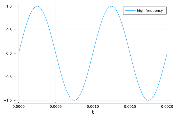
Fig. 102 A high frequency signal \(\sin(2 \pi t 1000)\).
Using SymPy.jl, we start defining the
low frequency and the high frequency signals:
lowfreq(t) = sin(2*pi*t/1000)
highfreq(t) = sin(2*pi*t*1000)
and then define the left of the ODE and the initial condition:
t = Sym("t")
y = SymFunction("y")
leftode = diff(y(t), t) + y(t)
initcond = Dict(y(0) => 0)
Then the right hand side for the low frequency signal:
filtlow = Eq(leftode, lowfreq(t))
outlow = dsolve(filtlow, ics=initcond)
The output for \(u(t) = u_{\rm low}(t) = \sin(2 \pi t/1000)\) is
For the high frequency signal we do:
filthigh = Eq(leftode, highfreq(t))
outhigh = dsolve(filthigh, ics=initcond)
The output for \(u(t) = u_{\rm high}(t) = \sin(2 \pi t 1000)\) is
The output for both signals is shown in Fig. 103 and in Fig. 104. We see that the low frequency signal passes, whereas the output of the high frequency signal is suppressed. The differential equation represents a lowpass filter.
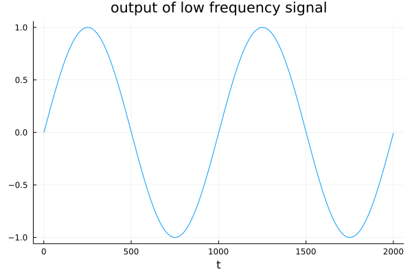
Fig. 103 The output of the low frequency signal \(\sin(2 \pi t/1000)\).
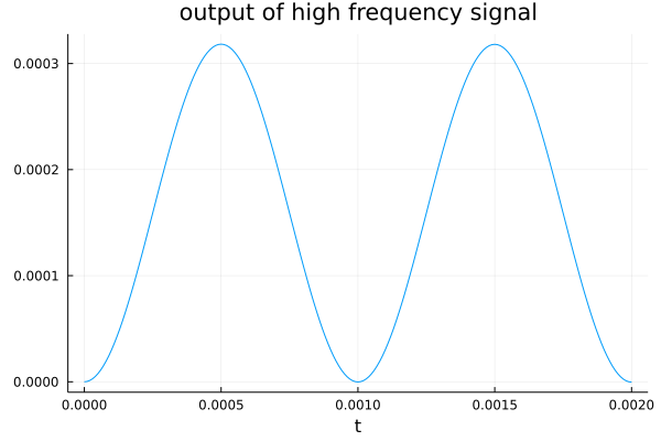
Fig. 104 The output of the high frequency signal \(\sin(2 \pi t 1000)\).
The first exercise considers a highpass filter.
A bandpass filter can be defined as a lowpass filter followed by highpass filter. Consider \(u(t)\) as input to
and then give \(y(t)\) as input to
which gives a bandpass filter. The frequency domain representation is
with \(Y(s) = {\cal L}\{ y \}\), \(U(s) = {\cal L}\{ u \}\), and \(Z(s) = {\cal L}\{ z \}\). This frequency domain representation is shown in Fig. 105.
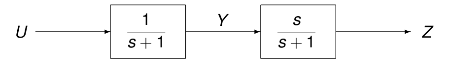
Fig. 105 Frequency domain representation of a bandpass filter.
This is an example of two cascading plants. We have that The transfer function of plants in cascade is the product of the transfer functions of the components in the cascade.
Electric Circuits
We consider the realization of lowpass and highpass filters as electric circuits.
The relation of voltage to current is shown in Fig. 106.
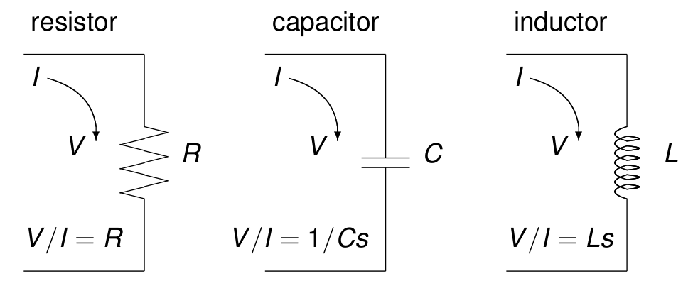
Fig. 106 The relation between the voltage \(v(t)\) across, and the current \(i(t)\) through a resistor, capacitor, and inductor.
Circuits are combined into networks, either by arranging them in series or in parallel, as shown in Fig. 107. If \(Z_1\) and \(Z_2\) are the transfer functions of two circuits, then the network defined by arranging the circuits in series has transfer function
If the circuits are arranged in parallel, then the transfer function of the network is

Fig. 107 Series and parallel circuits, with their transfer functions.
A circuit realization of a lowpass filter is shown in Fig. 108. For the resistor \(Z_1 = R\), and the capacitor \(Z_2 = \frac{1}{Cs}\), the transfer function of the realization in Fig. 108 is

Fig. 108 A realization of a lowpass filter.
In Fig. 109 is a circuit realization of a highpass filter. For the capacitor \(Z_1 = \frac{1}{Cs}\), and the resistor \(Z_2 = R\), the transfer function of the realization in Fig. 109 is

Fig. 109 A realization of a highpass filter.
Stability
In this section we develop a criterion to decide whether a plant is stable or not.
The inpulse response of a stable plant is decaying.
A criterion on the stability of a plant is provided by the theorem below.
For example, consider
The poles are \(-7/2 \pm \sqrt{33}/2\), so \(P\) is stable.
Two vehicle traffic is a situation where stability matters. Let \(u(t)\) be the position of the leading vehicle, and \(y(t)\) be the position of the trailing vehicle.
Modeling with an ordinary differential equation, with delay \(\tau\) and parameter \(\alpha\):
subject to the initial conditions \(y(0) = y'(0) = u(0) = u'(0) = 0\).
Integration leads to the differential equation:
In the frequency domain, we have:
This extends to the stability of following cars.
Proposal for a Topic of a Project
Consider the model for two vehicle traffic
Obtain the stability condition for this problem.
In particular, what is the relation between \(\tau\) and \(\alpha\) for this problem to be stable?
Show that even when stability is satisfied, a long platoon of vehicles is inherently unsafe because changes in speed of the lead car produce larger and larger deviations for cars farther down the platoon.
Exercises
The differential equation
\[\frac{d}{d~\!t} y(t) + y(t) = \frac{d}{d~\!t} u(t), \quad y(0) = 0\]is transformed into
\[s Y(s) + Y(s) = s U(s) \quad \Rightarrow \quad Y(s) = \left( \frac{s}{s+1} \right) U(s),\]where \(Y(s) = {\cal L}\{ y \}\) and \(U(s) = {\cal L}\{ u \}\).
Solve the above ODE for \(u = u_{\rm low}\) and \(u = u_{\rm high}\), that is: for a low and a high frequency signal, as defined earlier.
Verify that the ODE represents a highpass filter.
Consider a plant composed of
an inverting linear amplifier of gain \(-5\),
followed by an integrator \(\int_0^t\),
followed by a convolution with \(e^{-2t}\),
followed by a 3-second delay,
shown in Fig. 110.
Compute the time domain version of this cascading plant.
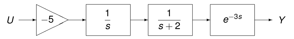
Fig. 110 An example of cascading plants.
Consider the network in Fig. 111.
Prove that the network has transfer function \(\displaystyle \frac{Y}{U} = \frac{Z_2}{Z_1 + Z_2}\).

Fig. 111 A network with input \(U\) and output \(Y\).
Let \(g(s) = a s^2 + b s + c\), with \(a, b, c > 0\).
What is the sign of the real parts of the roots of \(g\)?
Bibliography
Charles R. MacCluer, middle of Chapter 10 of Industrial Mathematics. Modeling in Industry, Science, and Government, Prentice Hall, 2000.
Richard C. Dorf and Robert H. Bishop: Modern Control Systems. Nineth Edition, Prentice Hall, 2001.