Filters and Feedback

Using continuous convolutions, we formulate the theorem on the gain and phase shift of a filter.

Filters

We study linear, time invariant, causal filters, viewed as plants, which also then provide mathematical models for mechanisms and filters. The linearity, time invariance, and causality imply that the respons of the unit impulse determines the behavior of the plant.

The convolution of two functions \(f\) and \(g\) is

\[f \star g = \int_0^t f(\tau) g(t - \tau) d \tau.\]

The Laplace transform takes a function from the time domain into the frequency domain. Considering filters:

• \(u(t)\) is the input signal, \(y(t)\) is the output signal,

• \(h(t)\) is the response of the unit impulse.

The convolution \(y = h \star u\) is transformed into

\[Y(s) = H(s) U(s), \quad U = {\cal L}\{ u \}, ~~ H = {\cal L}\{ h \}, ~~ Y = {\cal L}\{ y \},\]

where \(H(s)\) is the transfer function of the filter.

When designing a filter, we care about the gain and the phase shift.

Theorem on the gain and phase shift of a filter

Let \(H(s)\) be the transfer function of a filter. The response to \(u(t) = \sin(\omega t)\) is \(y(t) = r \sin(\omega t + \phi)\), where

• \(r(\omega) = | H(\omega i)|\) is the amplitude gain, and

• \(\phi(\omega) = \mbox{arg} H(\omega i)\) is the phase shift.

In applying the theorem, observe the following:

• For \(\omega = 2 \pi n\), the input signal \(u(t) = \sin(\omega t)\) runs at \(n\) Hertz.

• Complex numbers appear, the imaginary unit is \(i = \sqrt{-1}\).

• \(H(\omega i) \in {\mathbb C}\) and \(H(\omega i) = r e^{i \phi}\) is its polar representation.

In the proof of the theorem, we start with some complex arithmetic. Adding up

\[\begin{split}\begin{array}{lcr} e^{ i \omega t} & = & \cos(\omega t) + i \sin(\omega t) \\ - \left( e^{-i \omega t} \right. & = & \left. \vphantom{e^{i \omega t}} \cos(\omega t) - i \sin(\omega t) \right) \end{array}\end{split}\]

leads to

\[e^{i \omega t} - e^{-i \omega t} = 2 i \sin(\omega t).\]

Why this is useful:

\[\sin(\omega t) = \frac{1}{2i} \left( \vphantom{\frac{1}{2}} e^{i \omega t} - e^{-i \omega t} \right) \quad \Rightarrow \quad \mbox{we look at the response of } e^{i \omega t}.\]

Let us then look at the response of \(e^{i \omega t}\).

\[\begin{split}\begin{array}{rcl} y(t) & = & h(t) \star u(t) \\ & = & {\displaystyle \int_0^t h(\tau) e^{i \omega (t - \tau)} d \tau} \\ & = & {\displaystyle e^{i \omega t} \int_0^t h(\tau) e^{-i \omega \tau} d \tau} \\ & = & {\displaystyle e^{i \omega t} \left[ \int_0^\infty h(\tau) e^{-i \omega \tau} d \tau - \int_t^\infty h(\tau) e^{-i \omega \tau} d \tau \right]} \\ & & \mbox{\em Observe: } {\displaystyle \int_0^\infty h(\tau) e^{-s \tau} d \tau = {\cal L}\{ h \} = H(s).} \\ y(t) & = & e^{i \omega t} H(i \omega) + o(1) \end{array}\end{split}\]

The \(o(1)\) denotes a function with limit 0 as \(t \rightarrow \infty\).

Now we can study the response of \(\sin(\omega t)\). Applying \(y(t) = e^{i \omega t} H(i \omega)\), for \(u(t) = e^{i \omega t}\), to

\[\sin(\omega t) = \frac{1}{2i} \left( \vphantom{\frac{1}{2}} e^{i \omega t} - e^{-i \omega t} \right)\]

leads to

\[\begin{split}\begin{array}{rcl} h(t) \star \sin(\omega t) & = & {\displaystyle h(t) \star \frac{1}{2i} \left( \vphantom{\frac{1}{2}} e^{i \omega t} - e^{-i \omega t} \right)} \\ & = & {\displaystyle \frac{1}{2i} \left[ \vphantom{\frac{1}{2}} e^{i \omega t} H(i\omega) - e^{-i \omega t} H(-i \omega)\right]} \\ H(\omega i) \in {\mathbb C}: H(\omega i) = r e^{i \phi}: \quad & & \\ & = & {\displaystyle \frac{1}{2i} \left[ \vphantom{\frac{1}{2}} r e^{ i (\omega t + \phi)} - r e^{-i (\omega t + \phi)} \right]} \\ & = & r \sin\left( \vphantom{\frac{1}{2}} \omega t + \phi \right). \end{array}\end{split}\]

This finishes the proof.

An Application to Circuits

Fig. 111 Three circuits.

The three circuits in Fig. 111 have transfer functions, respectively:

\[\frac{Y}{U} = \frac{1}{1/Z_1 + 1/Z_2}, \quad \frac{Y}{U} = Z_1 + Z_2, \quad \mbox{and} \quad \frac{Y}{U} = \frac{Z_2}{Z_1 + Z_2}.\]

Fig. 112 A parallel resonant circuit.

Another example is shown in Fig. 112. With the notations for resistor: \(V/I = R\), inductor \(V/I = Ls\), capacitor: \(\displaystyle V/I = \frac{1}{Cs}\), the transfer function of the circuit in Fig. 112 is

\[\frac{Y}{U} = \frac{Z_2}{Z_1 + Z_2}, \quad Z_1 = R, \quad Z_2 = \frac{1}{\frac{1}{Ls} + Cs}.\]

The transfer functions allow to make the connection with ordinary differential equations. Expanding the transfer function

\[\frac{Y}{U} = \frac{Z_2}{Z_1 + Z_2}, \quad Z_1 = R, \quad Z_2 = \frac{1}{\frac{1}{Ls} + Cs}\]

into

\[\frac{\frac{Ls}{LC s^2 + 1}}{R + \frac{Ls}{LC s^2 + 1}} = \frac{Ls}{R L C s^2 + R + L s} = \frac{\frac{1}{RC} s}{s^2 + \frac{1}{R C} s + \frac{1}{L C}}\]

corresponds to the ordinary differential equation

\[y''(t) + \frac{1}{R C} y'(t) + \frac{1}{L C} = \frac{1}{R C} u'(t).\]

To see the effect of a filter, we consider its amplitude gain and phase shift. To apply the theorem on the gain and phase shift, we start with the transfer function, which is

\[H(s) = \frac{\frac{1}{RC} s}{s^2 + \frac{1}{R C} s + \frac{1}{L C}}.\]

Applying the theorem, we obtain \(r(\omega) = |H(\omega i)|\) is the amplitude gain, and \(\phi(\omega) = \mbox{arg} H(\omega i)\) is the phase shift. For the numerical plot, we use the following values for the two parameters: \(RC = 100/3\) and \(LC = 1/9\).

The code to make the Bode plot is below:

RC = 100/3; LC = 1/9
H(s) = ((1/RC)*s)/(s^2 + s/RC + 1/LC)
I = Complex(0, 1)

maxomega = 6
omegas = 0.01:0.01:maxomega

gains = [abs(H(I*w)) for w in omegas];
phases = [angle(H(I*w)) for w in omegas];

gainplot = plot(omegas, gains, xlabel="omega",
                ylabel = "gain", label = "")
phaseplot = plot(omegas, phases, xlabel="omega",
                 ylabel = "phase", label = "")
plot(gainplot, phaseplot)

The Bode plot is shown in Fig. 113.

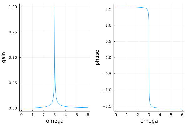
Fig. 113 The Bode plot of a peak filter.

Feedback

To introduce feedback, we consider the balance of a credit card:

• \(B_0\) is the initial balance,

• \(r\) is the annual interest rate,

• time \(t\) is measured in years.

In the time domain: \(B(t) = B_0 e^{r~\!t}\) as the solution of

\[\frac{d}{d~\!t} B(t) = r B(t), \quad B(0) = B_0.\]

Rewriting the ordinary differential equation:

\[\frac{d}{d~\!t} B(t) - r B(t) = 0 \quad \Leftrightarrow \quad (D - r) B = 0, \quad D = \frac{d}{d~\!t}.\]

In the frequency domain: \(\displaystyle P(s) = \frac{B_0}{s - r}\) is the transfer function. An open loop system is shown in Fig. 114.

Fig. 114 An open loop system.

For \(r > 0\), \(\displaystyle P(s) = \frac{B_0}{s - r}\) is unstable. Feedback can be used to stabilize a plant. A close loop system is shown in Fig. 115.

Fig. 115 A closed loop system.

The transfer function \(G(s)\) of the closed loop system is

\[G(s) = \frac{P(s)}{1 + P(s) H(s)},\]

as the input to \(P\) is

\[U(s) - H(s) Y(s)\]

and then

\[Y(s) = P(s) (U(s) - H(s) Y(s)) ~~ \Rightarrow ~~ (1 + P(s) H(s) ) Y(s) = P(s) U(s).\]

As an example of proportional feedback, consider \(\displaystyle P(s) = \frac{1}{s-1}\). A linear amplifier with gain \(\kappa\) has transfer function \(H(s) = \kappa\). The transfer function of the closed loop system is

\[G(s) = \frac{P(s)}{1 + P(s) H(s)} = \frac{1/(s-1)}{1 + \kappa/(s-1)} = \frac{1}{s + \kappa - 1}.\]

The closed loop system is stable for any \(\kappa > 1\).

Let us apply proportional feedback to paying off a credit card balance. Stabilize \(\displaystyle P(s) = \frac{B_0}{s - r}\) with proportional feedback \(\kappa\).

\[\begin{split}\begin{array}{rcl} G(s) & = & {\displaystyle \frac{P(s)}{1 + \kappa P(s)}} \\ & = & {\displaystyle \frac{\frac{B_0}{s - r}}{1 + \kappa \frac{B_0}{s-r}}} \\ & = & {\displaystyle \frac{B_0}{s - r + \kappa B_0}} \\ & = & {\displaystyle \frac{B_0}{s - (r - \kappa B_0)}} \end{array}\end{split}\]

The root of \(G(s)\) is \(r - \kappa B_0\). For stability: \(r < \kappa B_0\), or \(\kappa > r/B_0\).

Proposal for Topics of a Project

1. social feedback systems

   Supply and demand can be described via feedback.

   Read the paper by Otto Mayr on Adam Smith and the Concept of the Feedback System: Economic Thought and Technology in 18-th Century Britain in Technology and Culture, Volume 12, Number 1, 1971.

   Adam Smith suggested two processes:

   1. Workers compare various employments and stream into that employment which offers the greatest rewards.

   2. The rewards diminish as the number of competing workers rises.

   Do the following:

   • Use feedback to describe the labor market.

   • Apply your description to the academic labor market.

   • Find data comparing mathematics and computer science.

2. software for control systems

   Scilab and Xcos are open source software packages to design and analyze control systems.

   Visit <https://scilab.org>, download and install.

   Do the following:

   • Give an overview of the capabilities of the software.

   • Reproduce one of the use cases listed on the web site.

   • Write a report on your computational experiments.

Exercises

1. Is the filter \(y(t) = u(t/2)\) linear, causal, and time invariant? Justify your answer.

Fig. 116 Another realization of a filter.

2. Consider the circuit in Fig. 116.

   1. Derive the transfer function for this circuit.

   2. Write the corresponding ordinary differential equation.

3. Consider the transfer function

   \[H(s) = \frac{s^2 + 1}{s^2 + s + 1}.\]

   Make the Bode plot for \(\omega\) ranging between 0 and 0.5.

4. Consider the credit balance problem, with \(B_0 = \$1,000\), and \(r = 0.12\).

   • Examine the evolution of the balance paying \(\$50\) every month.

   • Interpret your examination relating to \(\kappa\).

Bibliography

1. Charles R. MacCluer, section 6 Chapter 10 of Industrial Mathematics. Modeling in Industry, Science, and Government, Prentice Hall, 2000.

2. Richard C. Dorf and Robert H. Bishop: Modern Control Systems. Nineth Edition, Prentice Hall, 2001.