Control, Root Locus, Nyquist Analysis

In this lecture, feedback control is introduced.

Control

We consider a plant \(P\), with controller \(H\), as shown in Fig. 117.

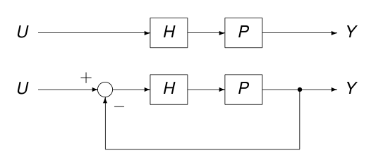
Fig. 117 The top picture represents an open loop system. The bottom piciture shows a closed loop system, obtained with feeding back the output to the input.

Feeding back the output to the input, an open loop system becomes a closed loop system. An example of feedback is steering control for an automobile.

In designing a servomechanism, we work with \(P(s) = 1/s\) as the transfer function of the plant. The controller has a transfer function \(H(s) = \kappa + \alpha/s\) and obtain a Proportional Integral (PI) controller. The problem is then to find the gains \(\kappa\) and \(\alpha\) that yield a step response with

• at most a \(20\%\) overshoot, and

• a 1-second rise time, the time to reach one.

For general plant with transfer function \(P\) and controller \(H\), the open loop function has transfer function \(H(s) P(s)\). The output is subtracted from the input in the closed loop:

\[Y(s) = H(s) P(s) ( U(s) - Y(s) ).\]

The transfer function of the closed loop system is then

\[(1 + H(s) P(s)) Y(s) = H(s) P(s) U(s) \quad \Rightarrow \quad \frac{Y(s)}{U(s)} = \frac{H(s)P(s)}{1 + H(s)P(s)}.\]

For the model of the servomechanism, \(P(s) = 1/s\). and \(H(s) = \kappa + \alpha/s\). The transfer function of the servomechanism is

\[G(s) = \frac{Y(s)}{U(s)} = \frac{H(s)P(s)}{1 + H(s)P(s)} = \frac{\kappa s + \alpha}{s^2 + \kappa s + \alpha}.\]

The response to the unit step is \(U(s) = 1/s\).

\[Y(s) = G(s) U(s) = \left( \frac{\kappa s + \alpha}{s^2 + \kappa s + \alpha} \right) \frac{1}{s} = \frac{1}{s} - \frac{s}{s^2 + \kappa s + \alpha}\]

We consider again :index: damped harmonic motion. The Laplace transform of the output of the unit step is

\[Y(s) = \frac{1}{s} - \frac{s}{s^2 + \kappa s + \alpha}.\]

The denominator is quadratic of \(Y(s)\), which corresponds to a second order differential equation. Substituting \(\kappa = 2 \zeta \omega_n\) and \(\alpha = \omega_n^2\) introduces the standard notation for damped harmonic motion:

\[Y(s) = \frac{1}{s} - \frac{s}{s^2 + 2 \zeta \omega_n s + \omega_n^2}.\]

which is equivalent to

\[Y(s) = \frac{1}{s} - \frac{s + \zeta \omega_n}{D} + \left( \frac{\zeta}{\sqrt{1 - \zeta^2}} \right) \frac{\omega_d}{D},\]

with

\[D = (s + \zeta \omega_n)^2 + \omega_d^2, \quad \omega_d = \sqrt{1 - \zeta^2} \omega_n.\]

Notice the distinction between \(\omega_n\) and \(\omega_d\).

To solve the ordinary differential equation, we apply the inverse Laplace transform, as done in the code below, executed in a Python session.

>>> from sympy import var
>>> from sympy import inverse_laplace_transform as ilap

>>> omega = var('omega', real=True)
>>> zeta = var('zeta', real=True)
>>> s, t = var('s, t')

>>> denominator = (s + zeta*omega)**2 + omega**2

>>> Y1 = - (s + zeta*omega)/denominator
>>> ilap(Y1, s, t)
-exp(-omega*t*zeta)*cos(omega*t)*Heaviside(t)

>>> Y2 = omega/denominator
>>> ilap(Y2, s, t)
exp(-omega*t*zeta)*sin(omega*t)*Heaviside(t)

Let us look at the output in the time domain. The inverse Laplace transform of

\[Y(s) = \frac{1}{s} - \frac{s + \zeta \omega_n}{D} + \left( \frac{\zeta}{\sqrt{1 - \zeta^2}} \right) \frac{\omega_d}{D},\]

with

\[D = (s + \zeta \omega_n)^2 + \omega_d^2, \quad \omega_d = \sqrt{1 - \zeta^2},\]

is then

\[\begin{split}\begin{array}{lcr} y(t) & = & {\displaystyle 1 - e^{-\zeta \omega_n t} \cos(\omega_d t) + \left( \frac{\zeta}{\sqrt{1 - \zeta^2}} \right) e^{-\zeta \omega_n t} \sin(\omega_d t)} \\ & = & {\displaystyle 1 - e^{-\zeta \omega_n t} \left[ \cos(\omega_d t) - \left( \frac{\zeta}{\sqrt{1 - \zeta^2}} \right) \sin(\omega_d t) \right].} \end{array}\end{split}\]

To determine the overshoot, we run simulations. The \(\zeta\) in the above solution for \(y(t)\) determines the overshoot, which should be less than \(20\%\). To study the effect of $zeta$, we go to normalized time

\[\tau = \omega_n t, \quad \omega_d = \sqrt{1 - \zeta^2},\]

and graph \(y(\tau)\), for various values of \(\zeta\), shown in Fig. 118, Fig. 119, and Fig. 120.

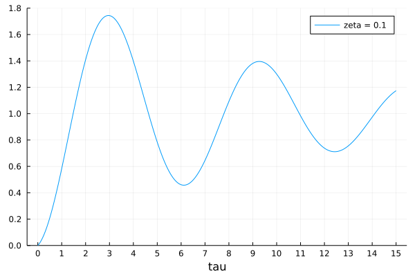
Fig. 118 A simulation for \(\zeta = 0.1\).

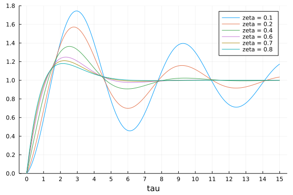
Fig. 119 Simulations for \(\zeta = 0.1, 0.2, 0.4, 0.6, 0.7, 0.8\).

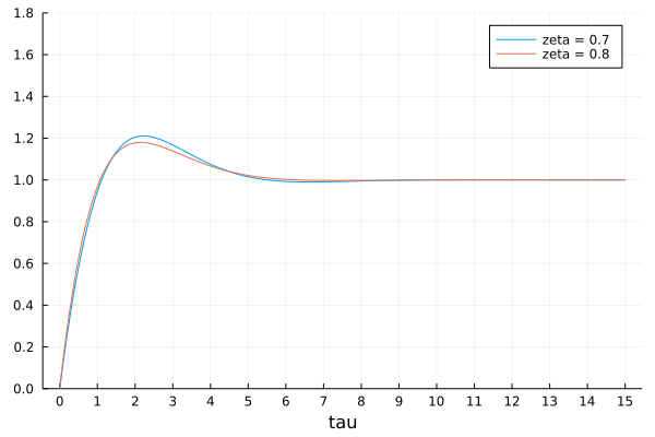
Fig. 120 Simulations for \(\zeta = 0.7, 0.8\).

Summarizing the observations from the simulations in Fig. 118, Fig. 119, and Fig. 120, gives a solution to the design problem.

• With \(\zeta = 0.7\), we go slightly above 1.2, so \(\zeta = 0.8\) is a safer value to meet the less than \(20\%\) overshoot.

• With \(\omega_n\), we can set the rise time, as \(\tau = \omega_n t\). For \(\zeta = 0.8\), at \(\tau = 1\), we reach 0.97, and 1.01 at \(\tau = 1.1\). If we want one at \(t=1\), then choose \(\omega = \tau/t = 1.1\).

• Use \(\kappa = 2 \zeta \omega_n = 1.76\) and \(\alpha = \omega_n^2 = 1.21\) in the design of the controller.

Root Locus

Consider a plant with transfer function

\[P(s) = \frac{s^2 + 7 s + 4}{s^3 - 3 s^2 + 2 s + 5}.\]

With proportional feedback \(H(s) = \kappa\), the closed loop system has transfer function

\[Q(s) = \frac{P}{1 + \kappa P}.\]

The denominator of \(Q(s)\) is

\[\kappa \left( s^2 + 7 s + 4 \right) + s^3 - 3 s^2 + 2 s + 5.\]

The closed loop system is stable if and only if all roots of the denominator all lie in the open left plane \(\mbox{real}(s) < 0\).

We apply the root locus method, using SymPy, in a Julia function defined below:

"""
    function locus(kp::Float64, p)

returns the roots of the polynomial p in s defined by
the coefficients where kappa is replaced by kp.
"""
function locus(kp::Float64, p)
    cffs = [p.coeff(s,k) for k=0:3]
    c1 = [c.subs(Dict(kappa=>kp)) for c in cffs]
    cf1 = [Float64(c1[k]) for k=1:size(c1,1)]
    p1s = sum([cf1[k]*s^(k-1) for k=1:size(cf1,1)])
    r1 = roots(p1s)
    v1 = [Float64(real(r[1]))+Float64(imag(r[1]))*Complex(0,1)
          for r in r1]
    tripletsort!(v1)
    return v1
end

The function tripletsort!(v1) sorts the numbers in v1.

The output of runs with this function is shown in Fig. 121, Fig. 122, and Fig. 123.

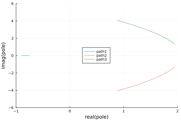
Fig. 121 The poles for \(\kappa = 2\), unstable.

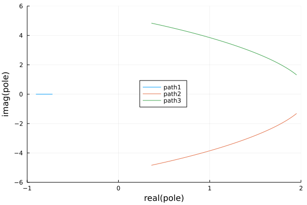
Fig. 122 The poles for \(\kappa = 3\), still unstable.

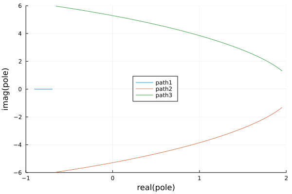
Fig. 123 The poles for \(\kappa = 5\), stable.

Nyquist analysis

The stability of the closed loop system for proportional feedback is equivalent to finding a \(\kappa\) so that the roots of

\[\frac{1}{\kappa} + H(s) P(s) = 0\]

all lie in the open left half plane.

The method of Nyquist analysis operates as follows:

1. Set \(G(s) = H(s) P(s)\).

2. Graph the image \(\Gamma\) of \(z = G(s)\), for \(s = \omega i\), for increasing \(\omega\).

All \(\kappa\) so that \(-1/\kappa\) lies in the unbounded component of the z-plane disjointed by \(\Gamma\) will DEstabilize the closed loop system.

Consider the example:

\[P(s) = 1/(s-1), \quad H(s) = 1/(s-2), \quad G(s) = H(s) P(s).\]

The code to make the complex plot is below:

I = Complex(0, 1)
r(omega) = G(omega*I)
omegarange = -100:0.01:100
rt = [(real(r(t)), imag(r(t)))
       for r in omegarange]
plot(rt, xlabel="real part",
         ylabel="imag part", label="G(w*I)")

In Fig. 124, we see that the entire negative real axis is outside the curve. Thus, there is no \(\kappa > 0\) that stabilizes.

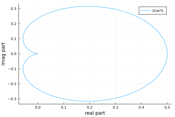
Fig. 124 The complex plot of \(1/((s-1)(s-2))\).

In Fig. 125, we see that, for another example, the entire negative real axis is outside the curve, except for \([-0.25, 0]\), so \(-1/\kappa \in [-0.25, 0]\) or \(\kappa > 4\), which agrees with the root locus method.

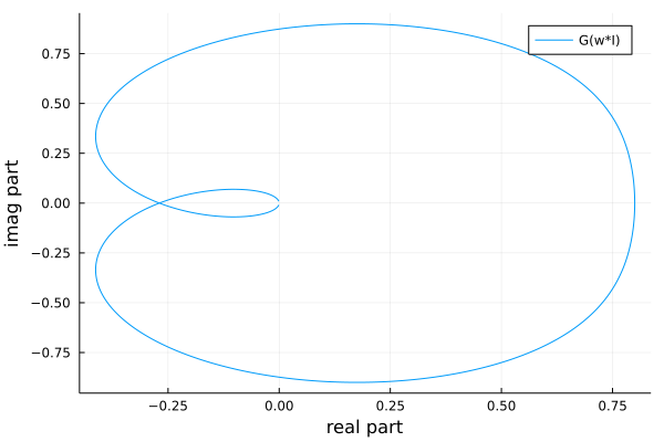
Fig. 125 The complex plot of \(G(s) = (s^2 + 7s + 4)/(s^3 - 3 s^2 + 2 s + 5)\).

We end with the argument principle.

Theorem on the argument principle

• Let \(\Omega\) be a domain in the complex plane.

• Suppose \(f(s)\) is meromorphic (analytic everywhere, except for poles) on \(\Omega\).

• Let \(C\) be the closed curve in \(\Omega\) that does not pass through any zeros or poles of \(f(s)\).

Then:

\[\frac{1}{2 \pi i} \int_C \frac{f'(s)}{f(s)} ds = \#\mbox{zeros} - \#\mbox{poles}\]

in \(\Omega\) enclosed by \(C\), counted with multiplicities.

As a corollary, the winding number \(n(z_0, C)\) counts the number of roots minus the number of poles of \(f(s) - z_0 = 0\) within \(C\).

Definition of the Nyquist contour

For \(R>0\), the Nyquist contour is

1. the imaginary axis from \(-R i\) to \(+R i\), and

2. the semi-circle \(R e^{i \theta}\), for \(\theta\) from \(+\pi/2\) to \(-\pi/2\).

To check the stability of a rational plant \(P(s) = N(s)/D(s)\), check that no poles of \(P\) lie within the Nyquist contour for large \(R\).

Proposals for a Topic of a Project

1. design an automobile cruise control system

   Our text book has the design of an automobile cruise control system. Study the solution to this design problem in our text book.

   Do the following:

   • Describe the solution using your own words.

   • Do the computational experiments to examine the stability.

   • Write a report on your computational experiments.

2. root finding with the winding number

   The winding number leads to a numerical method to approximate all roots of a general nonlinear equation in a domain of the complex plane.

   Study the proof of the argument principle theorem in our text book and make sure you understand the definition of the winding number.

   Do the following:

   • Describe the algorithm to compute all complex roots in a domain of a general nonlinear function.

   • Experiment with the implementation in Pari/GP.

   • Write a report on your computational experiments.

Exercises

1. Apply the partial fraction decomposition to justify

   \[\left( \frac{\kappa s + \alpha}{s^2 + \kappa s + \alpha} \right) \frac{1}{s} = \frac{1}{s} - \frac{s}{s^2 + \kappa s + \alpha}.\]

2. For the root locus example, find the critical threshold for \(\kappa\), so the closed loop system is stable when \(\kappa\) crosses this threshold.

3. The function locus is inefficient and tripletsort! a hack.

   A continuation method operates in two stages:

   • Update \(\kappa\) as \(\kappa + \Delta \kappa\), with step size \(\Delta \kappa\).

   • After each update, apply Newton’s method to correct the root.

   Apply this continuation method on the example of the root locus method.

Bibliography

1. Charles R. MacCluer, end of Chapter 10 of Industrial Mathematics. Modeling in Industry, Science, and Government, Prentice Hall, 2000.

2. Richard C. Dorf and Robert H. Bishop: Modern Control Systems. Nineth Edition, Prentice Hall, 2001.