Programming GPUs with PyCUDA and Julia

High level GPU programming can be done in Python or Julia. Before introducing PyCUDA and GPU programming with Julia, the data parallel model is described.

Data Parallelism

The programming model is Single Instruction Multiple Data (SIMD). In the application of data parallelism, blocks of threads read from memory, execute the same instruction(s), and then write the results back to memory. To fully occupy a massively parallel processor such as the GPU, at least 10,000 threads are needed.

Code that runs on the GPU is defined in a function, the so-called kernel.

The scalable programming model of the GPU is illustrated in Fig. 53.

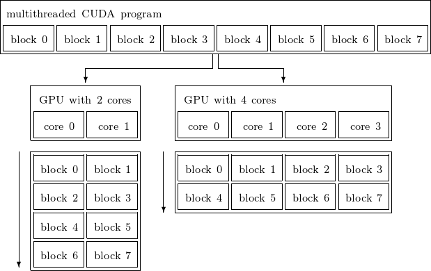
Fig. 53 A scalable programming model. Each core represents a streaming multiprocessor.

Streaming multiprocessors schedule the blocks of threads for execution in groups of 32 threads, called a warp. The dual warp scheduler is illustrated in Fig. 54.

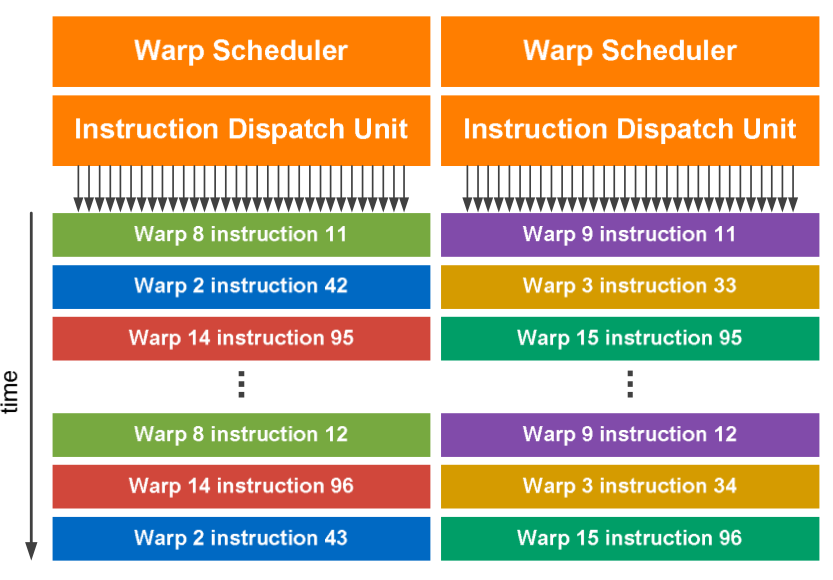
Fig. 54 Dual warp scheduler, copied from the NVIDIA documentation.

A kernel launch creates a grid of blocks, and each block has one or more threads. The organization of the grids and blocks can be 1D, 2D, or 3D. During the running of the kernel, threads in the same block are executed simultaneously.

The programming model for NVIDIA GPUs is called CUDA which stands for Compute Unified Device Architecture.

Programming GPUs is more complicated because it is not possible to quickly add print statements when debugging the code. As illustrated in Fig. 55 every GPU (called the device) is connected to a CPU (called the host). Kernels are lauched by the host for execution on the device.

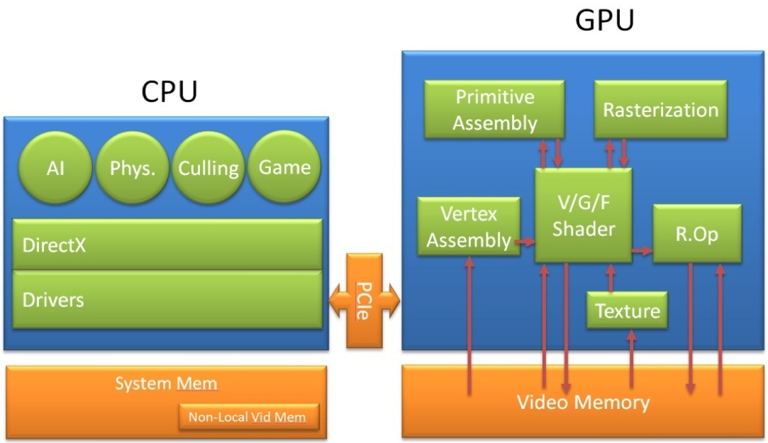
Fig. 55 From the GeForce 8 and 9 Series GPU Programming Guide (NVIDIA).

Matrix Matrix Multiplication

Our scientific running example of data parallel computations is the multiplication of two matrices. Consider the multiplication of matrices \(A\) and \(B\) which results in \(C = A \cdot B\), with

\[A = [a_{i,j}] \in {\mathbb R}^{n \times m}, \quad B = [b_{i,j}] \in {\mathbb R}^{m \times p}, \quad C = [c_{i,j}] \in {\mathbb R}^{n \times p}.\]

\(c_{i,j}\) is the inner product of the i-th row of \(A\) with the j-th column of \(B\):

\[c_{i,j} = \sum_{k=1}^m a_{i,k} \cdot b_{k,j}.\]

All \(c_{i,j}\)’s can be computed independently from each other. For \(n = m = p = 1,024\) we have 1,048,576 inner products. The matrix multiplication is illustrated in Fig. 56.

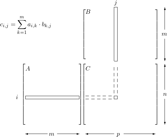
Fig. 56 Data parallelism in matrix multiplication.

PyCUDA

Code for the GPU can be generated in Python, see Fig. 57, as described in the following paper by A. Kloeckner, N. Pinto, Y. Lee, B. Catanzaro, P. Ivanov, and A. Fasih: PyCUDA and PyOpenCL: A scripting-based approach to GPU run-time code generation. Parallel Computing, 38(3):157–174, 2012.

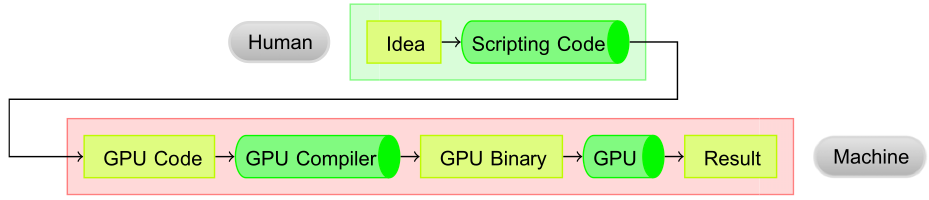
Fig. 57 The operating principle of GPU code generation.

To verify whether PyCUDA is correctly installed on our computer, we can run an interactive Python session as follows.

>>> import pycuda
>>> import pycuda.autoinit
>>> from pycuda.tools import make_default_context
>>> c = make_default_context()
>>> d = c.get_device()
>>> d.name()
'Tesla P100-PCIE-16GB'

We illustrate the matrix-matrix multiplication on the GPU with code generated in Python. We multipy an n-by-m matrix with an m-by-p matrix with a two dimensional grid of \(n \times p\) threads. For testing we use 0/1 matrices.

$ python matmatmul.py
matrix A:
[[ 0.  0.  1.  0.]
 [ 0.  0.  1.  1.]
 [ 0.  1.  1.  0.]]
matrix B:
[[ 1.  1.  0.  1.  1.]
 [ 1.  0.  1.  0.  0.]
 [ 0.  0.  1.  1.  0.]
 [ 0.  0.  1.  1.  0.]]
multiplied A*B:
[[ 0.  0.  1.  1.  0.]
 [ 0.  0.  2.  2.  0.]
 [ 1.  0.  2.  1.  0.]]
$

The script starts with the import of the modules and type declarations.

import pycuda.driver as cuda
import pycuda.autoinit
from pycuda.compiler import SourceModule
import numpy

(n, m, p) = (3, 4, 5)

n = numpy.int32(n)
m = numpy.int32(m)
p = numpy.int32(p)

a = numpy.random.randint(2, size=(n, m))
b = numpy.random.randint(2, size=(m, p))
c = numpy.zeros((n, p), dtype=numpy.float32)

a = a.astype(numpy.float32)
b = b.astype(numpy.float32)

The script then continues with the memory allocation and the copying from host to device.

a_gpu = cuda.mem_alloc(a.size * a.dtype.itemsize)
b_gpu = cuda.mem_alloc(b.size * b.dtype.itemsize)
c_gpu = cuda.mem_alloc(c.size * c.dtype.itemsize)

cuda.memcpy_htod(a_gpu, a)
cuda.memcpy_htod(b_gpu, b)

The definition of the kernel follows:

mod = SourceModule("""
    __global__ void multiply
      ( int n, int m, int p,
        float *a, float *b, float *c )
    {
        int idx = p*threadIdx.x + threadIdx.y;

        c[idx] = 0.0;
        for(int k=0; k<m; k++)
           c[idx] += a[m*threadIdx.x+k]
                    *b[threadIdx.y+k*p];
    }
    """)

To understand the code in the kernel, observe that a linear address system is used for the 2-dimensional array. Consider a 3-by-5 matrix stored row-wise (as in C), as shown in Fig. 58.

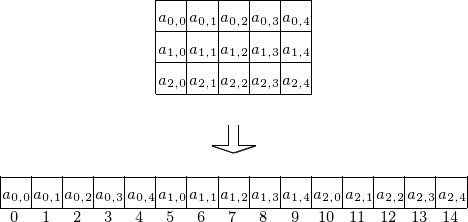
Fig. 58 Storing a matrix as a one dimensional array.

When defining the kernel, we assign inner products to threads. For example, consider a 3-by-4 matrix \(A\) and a 4-by-5 matrix \(B\), as in Fig. 59.

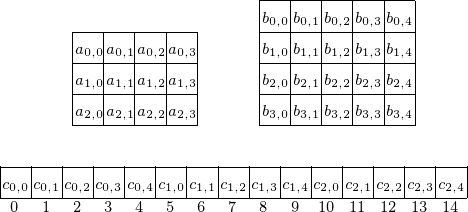
Fig. 59 Assigning inner products to threads.

The i = blockIdx.x*blockDim.x + threadIdx.x determines what entry in \(C = A \cdot B\) will be computed:

• the row index in \(C\) is i divided by 5 and

• the column index in \(C\) is the remainder of i divided by 5.

The launching of the kernel and printing the result is the last stage.

func = mod.get_function("multiply")
func(n, m, p, a_gpu, b_gpu, c_gpu, \
     block=(int(n), int(p), 1), \
     grid=(1, 1), shared=0)

cuda.memcpy_dtoh(c, c_gpu)

print("matrix A:")
print(a)
print("matrix B:")
print(b)
print("multiplied A*B:")
print(c)

Vendor Agnostic GPU Computing in Julia

The package CUDA.jl allows GPU programming in Julia, on computers with an NVIDIA GPU and provided that the CUDA Software Development Kit is installed. The compilation process for Julia is illustrated in Fig. 60.

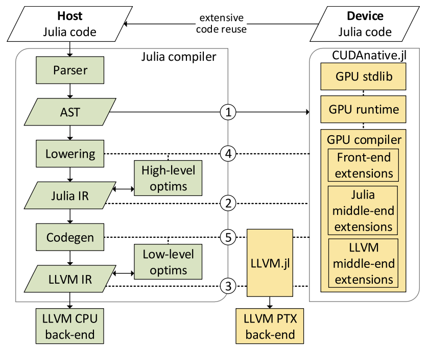
Fig. 60 The compilation process, copied from Besard et al., 2019.

The site JuliaGPU documents the organization to unify the many packages for programming GPUs in Julia. A first kernel is taken from the tutorials at the JuliaGPU site:

using CUDA
using Test

function gpu_add1!(y, x)
    for i = 1:length(y)
        @inbounds y[i] += x[i]
    end
    return nothing
end

N = 2^20             # adding one million Float32 numbers
x_d = CUDA.fill(1.0f0, N) # stored on GPU filled with 1.0
y_d = CUDA.fill(2.0f0, N) # stored on GPU filled with 2.0

fill!(y_d, 2)
@cuda gpu_add1!(y_d, x_d)
result = (@test all(Array(y_d) .== 3.0f0))
println(result)

Observe that, unlike with PyCUDA, the kernel is defined as a Julia function.

To make the point of {vendor agnostic GPU computing, in addition to CUDA.jl, the following packages are available:

• AMDGPU.jl for AMD GPUs,

• oneAPI.jl for the Intel oneAPI,

• Metal.jl to program GPUs in Apple hardware.

The code to add vectors on an M1 MacBook Air GPU with Metal looks very similar to the code with CUDA.jl.

using Metal
using Test

function gpu_add1!(y, x)
    for i = 1:length(y)
        @inbounds y[i] += x[i]
    end
    return nothing
end

N = 32
x_d = Metal.fill(1.0f0, N)  # filled with Float32 1.0 on GPU
y_d = Metal.fill(2.0f0, N)  # filled with Float32 2.0

# run with N threads

@metal threads=N gpu_add1!(y_d, x_d)
result = (@test all(Array(y_d) .== 3.0f0))

println(result)

As a last illustration, consider the multiplying of matrices with Metal. The CUDA version of the example is copied from the Julia for High-Performance Scientific Computing web site, adjusted

1. using Metal instead of using CUDA,

2. work with Float32 instead of Float64,

3. use MtlArray instead of CuArray.

The code is below, using the operator *:

using Metal
using BenchmarkTools

dim = 2^10
A_h = rand(Float32, dim, dim);
A_d = MtlArray(A_h);

@btime $A_h * $A_h;
@btime $A_d * $A_d;

When executed on a 2020 M1 Macbook Air, what is printed is 6.229 ms and 23.625 \(\mu\mbox{s}\) for CPU and GPU respectively. Observe the difference in orders of magnitude, milliseconds versus microseconds. Even as the GPU on this laptop is not intended for high performance scientific computations, it outperforms the CPU.

Bibliography

1. T. Besard, C. Foket, and B. De Sutter: Effective Extensible Programming: Unleashing Julia on GPUs. IEEE Transactions on Parallel and Distributed Systems, Vol. 30, No. 4, pages 827–841, 2019.

2. A. Kloeckner, N. Pinto, Y. Lee, B. Catanzaro, P. Ivanov, and A. Fasih. PyCUDA and PyOpenCL: A scripting-based approach to GPU run-time code generation. Parallel Computing, 38(3):157–174, 2012.

3. U. Utkarsh, V. Churavy, Y. Ma, T. Besard, P. Srisuma, T. Gymnich, A. R. Gerlach, A. Edelman, G. Barbastathis, R. D. Braatz, and C. Rackauckas: Automated Translation and Accelerated Solving of Differential Equations on Multiple GPU Platforms. Computer Methods in Applied Mechanics and Engineering, Vol. 419, 2024, article 116591.

Exercises

1. The matrix matrix multiplication example with PyCUDA uses \((3, 4, 5)\) as values for \((n, m, p)\). Considering massive parallelism, what are the largest dimensions you could consider for one block of threads on the P100 and/or the A100? Illustrate your values for the dimensions experimentally.

2. In the PyCUDA matrix matrix multiplication, change the float32 types into float64 and redo the previous exercise. Time the code. Do you notice a difference?

3. On your own computer, check the vendor of the GPU and run the equivalent gpuadd.jl after installing the proper Julia package. Report on the performance, relative to the CPU in your computer.