Warps and Reduction Algorithms

We discuss warp scheduling, latency hiding, SIMT, and thread divergence. To illustrate the concepts we discussed two reduction algorithms.

More on Thread Execution

The grid of threads are organized in a two level hierarchy:

• the grid is 1D, 2D, or 3D array of blocks; and

• each block is 1D, 2D, or 3D array of threads.

Blocks can execute in any order. Threads are bundled for execution. Each block is partitioned into warps.

Definition of warp

A warp is a unit of 32 threads, executed simultaneously by a streaming multiprocessor.

On the Tesla C2050/C2070, K20C, P100, V100, and A100, each warp consists of 32 threads.

The scheduling of threads is represented schematically in Fig. 72.

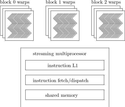
Fig. 72 Scheduling of threads by a streaming multiprocessor.

Let us consider the thread indices of warps. All threads in the same warp run at the same time. The partitioning of threads in a one dimensional block, for warps of size 32:

• warp 0 consists of threads 0 to 31 (value of threadIdx),

• warp \(w\) starts with thread \(32w\) and ends with thread \(32(w+1)-1\),

• the last warp is padded so it has 32 threads.

In a two dimensional block, threads in a warp are ordered along a lexicographical order of (threadIdx.x, threadIdx.y). For example, an 8-by-8 block has 2 warps (of 32 threads):

• warp 0 has threads \((0,0), (0,1), \ldots, (0,7)\), \((1,0), (1,1), \ldots, (1,7)\), \((2,0), (2,1), \ldots, (2,7)\), \((3,0), (3,1), \ldots, (3,7)\); and

• warp 1 has threads \((4,0), (4,1), \ldots, (4,7)\), \((5,0), (5,1), \ldots, (5,7)\), \((6,0), (6,1), \ldots, (6,7)\), \((7,0), (7,1), \ldots, (7,7)\).

As shown in Fig. 54, each streaming multiprocessor of the Fermi architecture has a dual warp scheduler.

Why give so many warps to a streaming multiprocessor if there only 32 can run at the same time? The answer is to efficiently execute long latency operations. What is this latency?

• A warp must often wait for the result of a global memory access and is therefore not scheduled for execution.

• If another warp is ready for execution, then that warp can be selected to execute the next instruction.

Definition of latency hiding

The mechanism of filling the latency of an expensive operation with work from other threads is known as latency hiding.

Warp scheduling is used for other types of latency operations, for example: pipelined floating point arithmetic and branch instructions. With enough warps, the hardware will find a warp to execute, in spite of long latency operations. The selection of ready warps for execution introduces no idle time and is referred to as zero overhead thread scheduling. The long waiting time of warp instructions is hidden by executing instructions of other warps. In contrast, CPUs tolerate latency operations with cache memories, and branch prediction mechanisms.

Let us consider how this applies to matrix-matrix multiplication For matrix-matrix multiplication, what should the dimensions of the blocks of threads be? We narrow the choices to three: \(8 \times 8\), \(16 \times 16\), or \(32 \times 32\)?

Considering that the C2050/C2070 has 14 streaming multiprocessors:

1. \(32 \times 32 = 1,024\) equals the limit of threads per block.

2. \(8 \times 8 = 64\) threads per block and \(1,024/64 = 12\) blocks.

3. \(16 \times 16 = 256\) threads per block and \(1,024/256 = 4\) blocks.

Note that we must also take into account the size of shared memory when executing tiled matrix matrix multiplication.

In multicore CPUs, we use Single-Instruction, Multiple-Data (SIMD): the multiple data elements to be processed by a single instruction must be first collected and packed into a single register.

In SIMT, all threads process data in their own registers. In SIMT, the hardware executes an instruction for all threads in the same warp, before moving to the next instruction. This style of execution is motivated by hardware costs constraints. The cost of fetching and processing an instruction is amortized over a large number of threads.

Single-Instruction, Multiple-Thread works well when all threads within a warp follow the same control flow path. For example, for an if-then-else construct, it works well

• when either all threads execute the then part,

• or all execute the else part.

If threads within a warp take different control flow paths, then the SIMT execution style no longer works well.

Considering the if-then-else example, it may happen that

• some threads in a warp execute the then part,

• other threads in the same warp execute the else part.

In the SIMT execution style, multiple passes are required:

• one pass for the then part of the code, and

• another pass for the else part.

These passes are sequential to each other and thus increase the execution time.

Definition of thread divergence

If threads in the same warp follow different paths of control flow, then we say that these threads diverge in their execution.

Next are other examples of thread divergence. Consider an iterative algorithm with a loop some threads finish in 6 iterations, other threads need 7 iterations. In this example, two passes are required: * one pass for those threads that do the 7th iteration, * another pass for those threads that do not.

In some code, decisions are made on the threadIdx values:

• For example: if(threadIdx.x > 2){ ... }.

• The loop condition may be based on threadIdx.

An important class where thread divergence is likely to occur is the class of reduction algorithms.

Parallel Reduction Algorithms

Typical examples of reduction algorithms are the computation of the sum or the maximum of a sequence of numbers. Another example is a tournament, shown in Fig. 73. A reduction algorithm extracts one value from an array, e.g.: the sum of an array of elements, the maximum or minimum element in an array. A reduction algorithm visits every element in the array, using a current value for the sum or the maximum/minimum. Large enough arrays motivate parallel execution of the reduction. To reduce \(n\) elements, \(n/2\) threads take \(\log_2(n)\) steps.

Reduction algorithms take only 1 flop per element loaded. They are

• not compute bound, that is: limited by flops performance,

• but memory bound, that is: limited by memory bandwidth.

When judging the performance of code for reduction algorithms, we have to compare to the peak memory bandwidth and not to the theoretical peak flops count.

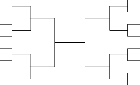
Fig. 73 A example of a reduction: a tournament.

As an introduction to a kernel for the parallel sum, consider the summation of 32 numbers, see Fig. 74.

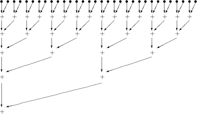
Fig. 74 Summing 32 numbers in a parallel reduction.

The original array is in the global memory and copied to shared memory for a thread block to sum. A code snippet in the kernel to sum number follows.

__shared__ float partialSum[];

int t = threadIdx.x;
for(int stride = 1; stride < blockDim.x; stride *= 2)
{
   __syncthreads();
   if(t % (2*stride) == 0)
      partialSum[t] += partialSum[t+stride];
}

The reduction is done in place, replacing elements. The __syncthreads() ensures that all partial sums from the previous iteration have been computed.

Because of the statement

if(t % (2*stride) == 0)
   partialSum[t] += partialSum[t+stride];

the kernel clearly has thread divergence. In each iteration, two passes are needed to execute all threads, even though fewer threads will perform an addition. Let us see if we can develop a kernel with less thread divergence.

Consider again the example of summing 32 numbers, but now with a different organization, as shown in Fig. 75.

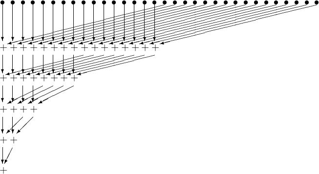
Fig. 75 The parallel summation of 32 number revised.

The original array is in the global memory and copied to shared memory for a thread block to sum. The kernel for the revised summation is below.

__shared__ float partialSum[];

int t = threadIdx.x;
for(int stride = blockDim.x >> 1; stride > 0;
    stride >> 1)
{
   __syncthreads();
   if(t < stride)
      partialSum[t] += partialSum[t+stride];
}

The division by 2 is done by shifting the stride value to the right by 1 bit.

Why is there less thread divergence? Af first, there seems no improvement, because of the if. Consider a block of 1,024 threads, partitioned in 32 warps. A warp consists of 32 threads with consecutive threadIdx values:

• all threads in warp 0 to 15 execute the add statement,

• all threads in warp 16 to 31 skip the add statement.

All threads in each warp take the same path \(\Rightarrow\) no thread divergence. If the number of threads that execute the add drops below 32, then thread divergence still occurs. Thread divergence occurs in the last 5 iterations.

Julia Defined Kernels

The summing of 32 numbers in five steps with Metal on a M1 Macbook Air can be coded as below.

using Metal

"""
    function gpusum32!(a)

sums the 32 numbers in the array a.
On return a[1] contains the sum.
"""
function gpusum32!(a)
    i = thread_position_in_grid_1d()
    a[i] += a[i+16]
    a[i] += a[i+8]
    a[i] += a[i+4]
    a[i] += a[i+2]
    a[i] += a[i+1]
    return nothing
end

a_h = [convert(Float32, k) for k=1:32]
z_h = [0.0f0 for k=1:32] # padding with zeros
x_h = vcat(a_h, z_h)
println("the numbers to sum : ", x_h)
x_d = MtlArray(x_h)

@metal threads=32 gpusum32!(x_d)

println("the summed numbers : ", Array(x_d))

which prints the numbers 528.0, 527.0, 525.0, 522.0, etc.

The equivalent code to add 32 numbers in five steps with CUDA on an NVIDIA GPU is below.

using CUDA

"""
    function gpusum32!(a)

sums the 32 numbers in the array a.
On return a[1] contains the sum.
"""
function gpusum32!(a)
    i = threadIdx().x
    a[i] += a[i+16]
    a[i] += a[i+8]
    a[i] += a[i+4]
    a[i] += a[i+2]
    a[i] += a[i+1]
    return nothing
end

a_h = [convert(Float32, k) for k=1:32]
z_h = [0.0f0 for k=1:32] # padding with zeros
x_h = vcat(a_h, z_h)
println("the numbers to sum : ", x_h)
x_d = CuArray(x_h)

@cuda threads=32 gpusum32!(x_d)

println("the summed numbers : ", Array(x_d))

which prints the same numbers as in the other program.

To illustrate shared memory with CUDA.jl consider the summation of the first \(N\) natural numbers. The output of running firstsum.jl on an NVIDIA GPU is as follows:

$ julia firstsum.jl
size of the vector : 33792
  number of blocks : 32
 threads per block : 256
 number of threads : 8192
Does GPU value 570966528 = 570966528 ? true
$

In the check, we use \(\displaystyle \sum_{k=1}^N k = \frac{N (N+1)}{2}\). The definition of the kernel is below.

using CUDA

"""
    function sum(x, y, N, threadsPerBlock, blocksPerGrid)

computes the sum product of N numbers in x and
places the results in y, using shared memory.
"""
function sum(x, y, N, threadsPerBlock, blocksPerGrid)
    # set up shared memory cache for this current block
    cache = @cuDynamicSharedMem(Int64, threadsPerBlock)
    # initialise the indices
    tid = (threadIdx().x - 1) + (blockIdx().x - 1) * blockDim().x
    totalThreads = blockDim().x * gridDim().x
    cacheIndex = threadIdx().x - 1
    # run over the vector
    temp = 0
    while tid < N
        temp += x[tid + 1]
        tid += totalThreads
    end
    # set cache values
    cache[cacheIndex + 1] = temp
    # synchronise threads
    sync_threads()
    # we add up all of the values stored in the cache
    i::Int = blockDim().x ÷ 2
    while i!=0
        if cacheIndex < i
            cache[cacheIndex + 1] += cache[cacheIndex + i + 1]
        end
        sync_threads()
        i = i ÷ 2
    end
    # cache[1] now contains the sum of the numbers in the block
    if cacheIndex == 0
        y[blockIdx().x] = cache[1]
    end
    return nothing
end

The launching of the kernels happens in the main program below.

"""
    Tests the kernel on the first N natural numbers.
"""
function main()
    N::Int64 = 33 * 1024
    threadsPerBlock::Int64 = 256
    blocksPerGrid::Int64 = min(32, (N + threadsPerBlock - 1) / threadsPerBlock)
    println("size of the vector : ", N)
    println("  number of blocks : ", blocksPerGrid)
    println(" threads per block : ", threadsPerBlock)
    println(" number of threads : ", blocksPerGrid*threadsPerBlock)
    # input arrays on the host
    x_h = [i for i=1:N]
    # make the arrays on the device
    x_d = CuArray(x_h)
    y_d = CuArray(fill(0, blocksPerGrid))
    # execute the kernel. Note the shmem argument - this is necessary to allocate
    # space for the cache we allocate on the gpu with @cuDynamicSharedMem
    @cuda blocks = blocksPerGrid threads = threadsPerBlock shmem =
    (threadsPerBlock * sizeof(Int64)) sum(x_d, y_d, N, threadsPerBlock, blocksPerGrid)
    # copy the result from device to the host
    y_h = Array(y_d)
    local result = 0
    for i in 1:blocksPerGrid
        result += y_h[i]
    end
    # check whether output is correct
    print("Does GPU value ", result, " = ", N*(N+1) ÷ 2, " ? ")
    println(result == N*(N+1) ÷ 2)
end

Bibliography

• S. Sengupta, M. Harris, and M. Garland. Efficient parallel scan algorithms for GPUs. Technical Report NVR-2008-003, NVIDIA, 2008.

• M. Harris. Optimizing parallel reduction in CUDA. White paper available at <http://docs.nvidia.com>.

Exercises

1. Consider the code matrixMul of the GPU computing SDK. Look up the dimensions of the grid and blocks of threads. Can you (experimentally) justify the choices made?

2. Write code for the two summation algorithms we discussed. Do experiments to see which algorithm performs better.

3. Apply the summation algorithm to the composite trapezoidal rule. Use it to estimate \(\pi\) via \(\displaystyle \frac{\pi}{4} = \int_0^1 \sqrt{1-x^2} dx\).