Pipelined Sorting, Sieving, Substitution
We continue our study of pipelined computations, for sorting, prime number generation, and solving triangular linear systems.
Sorting Numbers
As a data archival application, consider a pipeline with four computers in Fig. 85.
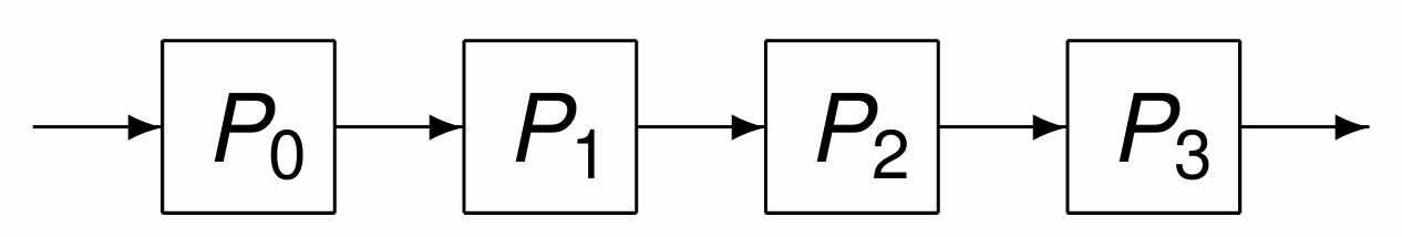
Fig. 85 A 4-stage pipeline in a data archival application.
The most recent data is stored on \(P_0\).
When \(P_0\) receives new data, its older data is moved to \(P_1\).
When \(P_1\) receives new data, its older data is moved to \(P_2\).
When \(P_2\) receives new data, its older data is moved to \(P_3\).
When \(P_3\) receives new data, its older data is archived to tape.
This is a type 1 pipeline. Every processor does the same three steps:
receive new data,
sort data,
send old data.
medskip
This leads to a pipelined sorting of numbers.
We consider a parallel version of insertion sort,
sorting p numbers with p processors.
Processor i does p-i steps in the algorithm:
for step 0 to p-i-1 do
    manager receives number
    worker i receives number from i-1
    if step = 0 then
       initialize the smaller number
    else if number > smaller number then
       send number to i+1
    else
       send smaller number to i+1;
       assign number to smaller number;
    end if;
end for.
A pipeline session with MPI can go as below.
$ mpirun -np 4 /tmp/pipe_sort
The 4 numbers to sort :  24 19 25 66
Manager gets 24.
Manager gets 19.
Node 0 sends 24 to 1.
Manager gets 25.
Node 0 sends 25 to 1.
Manager gets 66.
Node 0 sends 66 to 1.
Node 1 receives 24.
Node 1 receives 25.
Node 1 sends 25 to 2.
Node 1 receives 66.
Node 1 sends 66 to 2.
Node 2 receives 25.
Node 2 receives 66.
Node 2 sends 66 to 3.
Node 3 receives 66.
The sorted sequence :  19 24 25 66
MPI code for a pipeline version of insertion sort is in
the program pipe_sort.c below:
int main ( int argc, char *argv[] )
{
   int i,p,*n,j,g,s;
   MPI_Status status;
   MPI_Init(&argc,&argv);
   MPI_Comm_size(MPI_COMM_WORLD,&p);
   MPI_Comm_rank(MPI_COMM_WORLD,&i);
   if(i==0) /* manager generates p random numbers */
   {
      n = (int*)calloc(p,sizeof(int));
      srand(time(NULL));
      for(j=0; j<p; j++) n[j] = rand() % 100;
      if(v>0)
      {
         printf("The %d numbers to sort : ",p);
         for(j=0; j<p; j++) printf(" %d", n[j]);
         printf("\n"); fflush(stdout);
      }
   }
   for(j=0; j<p-i; j++)  /* processor i performs p-i steps */
      if(i==0)
      {
         g = n[j];
         if(v>0) { printf("Manager gets %d.\n",n[j]); fflush(stdout); }
         Compare_and_Send(i,j,&s,&g);
      }
      else
      {
         MPI_Recv(&g,1,MPI_INT,i-1,tag,MPI_COMM_WORLD,&status);
         if(v>0) { printf("Node %d receives %d.\n",i,g); fflush(stdout); }
         Compare_and_Send(i,j,&s,&g);
      }
   MPI_Barrier(MPI_COMM_WORLD); /* to synchronize for printing */
   Collect_Sorted_Sequence(i,p,s,n);
   MPI_Finalize();
   return 0;
}
The function Compare_and_Send is defined next.
void Compare_and_Send ( int myid, int step, int *smaller, int *gotten )
/* Processor "myid" initializes smaller with gotten at step zero,
 * or compares smaller to gotten and sends the larger number through. */
{
   if(step==0)
      *smaller = *gotten;
   else
      if(*gotten > *smaller)
      {
         MPI_Send(gotten,1,MPI_INT,myid+1,tag,MPI_COMM_WORLD);
         if(v>0)
         {
            printf("Node %d sends %d to %d.\n",
                   myid,*gotten,myid+1);
            fflush(stdout);
         }
      }
      else
      {
         MPI_Send(smaller,1,MPI_INT,myid+1,tag,
                  MPI_COMM_WORLD);
         if(v>0)
         {
            printf("Node %d sends %d to %d.\n",
                   myid,*smaller,myid+1);
            fflush(stdout);
         }
         *smaller = *gotten;
      }
}
The function Collect_Sorted_Sequence follows:
void Collect_Sorted_Sequence ( int myid, int p, int smaller, int *sorted )
/* Processor "myid" sends its smaller number to the manager who collects
 * the sorted numbers in the sorted array, which is then printed. */
{
   MPI_Status status;
   int k;
   if(myid==0) {
      sorted[0] = smaller;
      for(k=1; k<p; k++)
         MPI_Recv(&sorted[k],1,MPI_INT,k,tag,
                  MPI_COMM_WORLD,&status);
      printf("The sorted sequence : ");
      for(k=0; k<p; k++) printf(" %d",sorted[k]);
      printf("\n");
   }
   else
      MPI_Send(&smaller,1,MPI_INT,0,tag,MPI_COMM_WORLD);
}
Prime Number Generation
The sieve of Erathostenes is shown in Fig. 86.
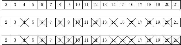
Fig. 86 Wiping out all multiples of 2 and 3 gives all prime numbers between 2 and 21.
A pipelined sieve algorithm is defined as follows. One stage in the pipeline
receives a prime,
receives a sequence of numbers,
extracts from the sequence all multiples of the prime, and
sends the filtered list to the next stage.
This pipeline algorithm is of type 2. As in type 1, multiple input items are needed for speedup; but the amount of work in every stage will complete fewer steps than in the preceding stage.
For example, consider a 2-stage pipeline to compute all primes \(\leq 21\) with the sieve algorithm:
wipe out all multiples of 2, in nine multiplications;
wipe out all multiples of 3, in five multiplications.
Although the second stage in the pipeline starts only after we determined that 3 is not a multiple of 2, there are fewer multiplications in the second stage. The space-time diagram with the multiplications is in Fig. 87.
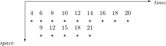
Fig. 87 A 2-stage pipeline to compute all primes \(\leq 21\).
A parallel implementation of the sieve of Erathostenes
is in the examples collection of the Intel TBB distribution,
in /usr/local/tbb40_20131118oss/examples/parallel_reduce/primes.
Computations on a 16-core computer kepler:
$ make
g++ -O2 -DNDEBUG  -o primes main.cpp primes.cpp -ltbb -lrt
./primes
#primes from [2..100000000] = 5761455 (0.106599 sec with serial code)
#primes from [2..100000000] = 5761455 (0.115669 sec with 1-way parallelism)
#primes from [2..100000000] = 5761455 (0.059511 sec with 2-way parallelism)
#primes from [2..100000000] = 5761455 (0.0393051 sec with 3-way parallelism)
#primes from [2..100000000] = 5761455 (0.0287207 sec with 4-way parallelism)
#primes from [2..100000000] = 5761455 (0.0237532 sec with 5-way parallelism)
#primes from [2..100000000] = 5761455 (0.0198929 sec with 6-way parallelism)
#primes from [2..100000000] = 5761455 (0.0175456 sec with 7-way parallelism)
#primes from [2..100000000] = 5761455 (0.0168987 sec with 8-way parallelism)
#primes from [2..100000000] = 5761455 (0.0127005 sec with 10-way parallelism)
#primes from [2..100000000] = 5761455 (0.0116965 sec with 12-way parallelism)
#primes from [2..100000000] = 5761455 (0.0104559 sec with 14-way parallelism)
#primes from [2..100000000] = 5761455 (0.0109771 sec with 16-way parallelism)
#primes from [2..100000000] = 5761455 (0.00953452 sec with 20-way parallelism)
#primes from [2..100000000] = 5761455 (0.0111944 sec with 24-way parallelism)
#primes from [2..100000000] = 5761455 (0.0107475 sec with 28-way parallelism)
#primes from [2..100000000] = 5761455 (0.0151389 sec with 32-way parallelism)
elapsed time : 0.520726 seconds
$
Solving Triangular Systems
We apply a type 3 pipeline to solve a triangular linear system. With forward substitution formulas we solve a lower triangular system.
The LU factorization of a matrix \(A\) reduces the solving of a linear system to solving two triangular systems. To solve an n-dimensional linear system \(A {\bf x} = {\bf b}\) we factor A as a product of two triangular matrices, \(A = L U\):
\(L\) is lower triangular, \(L = [\ell_{i,j}]\), \(\ell_{i,j} = 0\) if \(j > i\) and \(\ell_{i,i} = 1\).
\(U\) is upper triangular \(U = [u_{i,j}]\), \(u_{i,j} = 0\) if \(i > j\).
Solving \(A {\bf x} = {\bf b}\) is equivalent to solving \(L(U {\bf x}) = {\bf b}\):
Forward substitution: \(L {\bf y} = {\bf b}\).
Backward substitution: \(U {\bf x} = {\bf y}\).
Factoring \(A\) costs \(O(n^3)\), solving triangular systems costs \(O(n^2)\).
Expanding the matrix-vector product \(L {\bf y}\) in \(L {\bf y} = {\bf b}\) leads to formulas for forward substitution:
and solving for the diagonal elements gives
The formulas lead to an algorithm. For \(k=1,2,\ldots,n\):
Formulated as an algorithm, in pseudocode:
for k from 1 to n do
    y[k] := b[k]
    for i from 1 to k-1 do
        y[k] := y[k] - L[k][i]*y[i].
We count \(1 + 2 + \cdots + n-1 = \displaystyle \frac{n(n-1)}{2}\) multiplications and subtractions.
Pipelines are classified into three types:
Type 1: Speedup only if multiple instances. Example: instruction pipeline.
Type 2: Speedup already if one instance. Example: pipeline sorting.
Type 3: Worker continues after passing information through. Example: solve \(L {\bf y} = {\bf b}\).
Typical for the 3rd type of pipeline is the varying length of each job, as exemplified in Fig. 88.
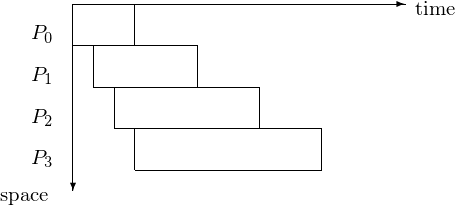
Fig. 88 Space-time diagram for pipeline with stages of varying length.
Using an n-stage pipeline, we assume that L is available on every processor.
The corresponding 4-stage pipeline is shown in Fig. 89 with the space-time diagram in Fig. 90.

Fig. 89 4-stage pipeline to solve a 4-by-4 lower triangular system.
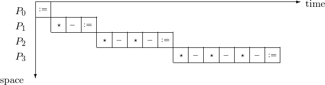
Fig. 90 Space-time diagram for solving a 4-by-4 lower triangular system.
In type 3 pipelining, a worker continues after passing results through. The making of \(y_1\) available in the next pipeline cycle is illustrated in Fig. 91. The corresponding space-time diagram is in Fig. 92 and the space-time diagram in Fig. 93 shows at what time step which component of the solution is.

Fig. 91 Passing \(y_1\) through the type 3 pipeline.
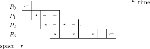
Fig. 92 Space-time diagram of a type 3 pipeline.
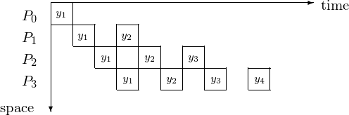
Fig. 93 Space-time diagram illustrates the component of the solutions.
We count the steps for \(p = 4\) or in general, for \(p = n\) as follows. The latency takes 4 steps for \(y_1\) to be at \(P_4\), or in general: n steps for \(y_1\) to be at \(P_n\). It takes then 6 additional steps for \(y_4\) to be computed by \(P_4\), or in general: \(2n-2\) additional steps for \(y_n\) to be computed by \(P_n\). So it takes \(n + 2n - 2 = 3n - 2\) steps to solve an n-dimensional triangular system by an n-stage pipeline.
y := b
for i from 2 to n do
    for j from i to n do
        y[j] := y[j] - L[j][i-1]*y[i-1]
Consider for example the solving of \(L {\bf y} = {\bf b}\) for \(n = 5\).
\(y := {\bf b}\);
\(y_2 := y_2 - \ell_{2,1} \star y_1\);
\(y_3 := y_3 - \ell_{3,1} \star y_1\);
\(y_4 := y_4 - \ell_{4,1} \star y_1\);
\(y_5 := y_5 - \ell_{5,1} \star y_1\);
\(y_3 := y_3 - \ell_{3,2} \star y_2\);
\(y_4 := y_4 - \ell_{4,2} \star y_2\);
\(y_5 := y_5 - \ell_{5,2} \star y_2\);
\(y_4 := y_4 - \ell_{4,3} \star y_3\);
\(y_5 := y_5 - \ell_{5,3} \star y_3\);
\(y_5 := y_5 - \ell_{5,4} \star y_4\);
Observe that all instructions in the j loop are independent from each other!
Consider the inner loop in the algorithm to solve \(L {\bf y} = {\bf b}\). We distribute the update of \(y_i, y_{i+1}, \ldots, y_n\) among p processors. If \(n \gg p\), then we expect a close to optimal speedup.
Bibliography
Shahid H. Bokhari. Multiprocessing the Sieve of Eratosthenes. Computer 20(4):50-58, 1987.
B. Wilkinson and M. Allen. Parallel Programming. Techniques and Applications Using Networked Workstations and Parallel Computers. Prentice Hall, 2nd edition, 2005.
Exercises
Write the pipelined sorting algorithm with OpenMP or Julia.
Demonstrate the correctness of your implementation with some good examples.
Use message passing to implement the pipelined sieve algorithm.
Relate the number of processors in the network to the number of multiples which must be computed before sending off the sequence to the next processor.
Implement the pipelined sieve algorithm with OpenMP and Julia.
Can the constraint on the number of computed multiples be formulated with dependencies?
Consider the upper triangular system \(U {\bf x} = {\bf y}\), with \(U = [u_{i,j}]\), \(u_{i,j} = 0\) if \(i > j\).
Derive the formulas and general algorithm to compute the components of the solution \({\bf x}\).
For \(n=4\), draw the third type of pipeline.