Solving Triangular Systems
Triangular linear system occur as the result of an LU or a QR decomposition.
Ill Conditioned Matrices and Quad Doubles
Consider the 4-by-4 lower triangular matrix
What we know from numerical analysis:
The condition number of a matrix magnifies roundoff errors.
The hardware double precision is \(2^{-52} \approx 2.2 \times 10^{-16}\).
We get no accuracy from condition numbers larger than \(10^{16}\).
An experiment in an interactive Julia session illustate that ill conditioned matrices occur already in modest dimensions.
julia> using LinearAlgebra

julia> A = ones(32,32);

julia> D = Diagonal(A);

julia> L = LowerTriangular(A);

julia> LmD = L - D;

julia> L2 = D - 2*LmD;

julia> cond(L2)
2.41631630569077e16
The condition number is estimated at \(2.4 \times 10^{16}\).
A floating-point number consists of a sign bit, exponent, and a fraction (also known as the mantissa). Almost all microprocessors follow the IEEE 754 standard. GPU hardware supports 32-bit (single float) and for compute capability \(\geq 1.3\) also double floats.
Numerical analysis studies algorithms for continuous problems, problems for their sensitivity to errors in the input; and algorithms for their propagation of roundoff errors.
The floating-point addition is not associative! Parallel algorithms compute and accumulate the results in an order that is different from their sequential versions. For example, adding a sequence of numbers is more accurate if the numbers are sorted in increasing order.
Instead of speedup, we can ask questions about quality up:
If we can afford to keep the total running time constant, does a faster computer give us more accurate results?
How many more processors do we need to guarantee a result?
A quad double is an unevaluated sum of 4 doubles,
improves the working precision from \(2.2 \times 10^{-16}\)
to \(2.4 \times 10^{-63}\).
The software QDlib is presented in the paper
Algorithms for quad-double precision floating point arithmetic
by Y. Hida, X.S. Li, and D.H. Bailey, published in the
15th IEEE Symposium on Computer Arithmetic, pages 155-162. IEEE, 2001.
The software is available at <http://crd.lbl.gov/~dhbailey/mpdist>.
A quad double builds on double double.
Some features of working with doubles double are:
The least significant part of a double double can be interpreted as a compensation for the roundoff error.
Predictable overhead: working with double double is of the same cost as working with complex numbers.
Consider Newton’s method to compute :math:sqrt{x}: as defined in the code below.
#include <iostream>
#include <iomanip>
#include <qd/qd_real.h>
using namespace std;

qd_real newton ( qd_real x )
{
   qd_real y = x;
   for(int i=0; i<10; i++)
      y -= (y*y - x)/(2.0*y);
   return y;
}
The main program is as follows.
int main ( int argc, char *argv[] )
{
   cout << "give x : ";
   qd_real x; cin >> x;
   cout << setprecision(64);
   cout << "        x : " << x << endl;

   qd_real y = newton(x);
   cout << "  sqrt(x) : " << y << endl;

   qd_real z = y*y;
   cout << "sqrt(x)^2 : " << z << endl;

   return 0;
}
If the program is in the file newton4sqrt.cpp
and the makefile contains
QD_ROOT=/usr/local/qd-2.3.13
QD_LIB=/usr/local/lib

newton4sqrt:
        g++ -I$(QD_ROOT)/include newton4sqrt.cpp \
              $(QD_LIB)/libqd.a -o /tmp/newton4sqrt
then we can create the executable,
simply typing make newton4sqrt.
A run with the code for \(sqrt{2}\) is shown below.
2.0000000000000000000000000000000000000000000000000000000000000000e+00
1.5000000000000000000000000000000000000000000000000000000000000000e+00
1.4166666666666666666666666666666666666666666666666666666666666667e+00
1.4142156862745098039215686274509803921568627450980392156862745098e+00
1.4142135623746899106262955788901349101165596221157440445849050192e+00
1.4142135623730950488016896235025302436149819257761974284982894987e+00
1.4142135623730950488016887242096980785696718753772340015610131332e+00
1.4142135623730950488016887242096980785696718753769480731766797380e+00
1.4142135623730950488016887242096980785696718753769480731766797380e+00
residual : 0.0000e+00
Accelerated Back Substitution
Consider a 3-by-3-tiled upper triangular system \(U {\bf x} = {\bf b}\).
where \(U_1\), \(U_2\), \(U_3\) are upper triangular, with nonzero diagonal elements.
Invert all diagonal tiles:
The inverse of an upper triangular matrix is upper triangular.
Solve an upper triangular system for each column of the inverse.
The columns of the inverse can be computed independently.
\(\Rightarrow\) Solve many smaller upper triangular systems in parallel.
After inverting the diagonal tiles, in the second stage, we solve \(U {\bf x} = {\bf b}\) for
in the following steps:
\({\bf x}_3 := U_3^{-1} {\bf b}_3\),
\({\bf b}_2 := {\bf b}_2 - A_{2,3} {\bf x}_3\), \({\bf b}_1 := {\bf b}_1 - A_{1,3} {\bf x}_3\),
\({\bf x}_2 := U_2^{-1} {\bf b}_2\),
\({\bf b}_1 := {\bf b}_1 - A_{1,2} {\bf x}_2\),
\({\bf x}_1 := U_1^{-1} {\bf b}_1\).
Statements on the same line can be executed in parallel. In multiple double precision, several blocks of threads collaborate in the computation of one matrix-vector product.
The two stages are executed by three kernels.
Algorithm 1: Tiled Accelerated Back Substitution.
On input are the following :
\(N\) is the number of tiles,
\(n\) is the size of each tile,
\(U\) is an upper triangular \(Nn\)-by-\(Nn\) matrix,
\({\bf b}\) is a vector of size \(Nn\).
The output is \(\bf x\) is a vector of size \(Nn\): \(U {\bf x} = {\bf b}\).
Let \(U_1, U_2, \ldots, U_N\) be the diagonal tiles.
The k-th thread solves \(U_i {\bf v}_k = {\bf e}_k\), computing the k-th column \(U^{-1}_i\).
For \(i=N, N-1, \ldots,1\) do
\(n\) threads compute \({\bf x}_i = U^{-1} {\bf b}_i\);
simultaneously update \({\bf b}_j\) with \({\bf b}_j - A_{j,i} {\bf x}_i\), \(j \in \{1,2,\ldots,i-1\}\) with \(i-1\) blocks of \(n\) threads.
A parallel execution could run in time proportional to \(N n\).
For efficiency, we must stage the data right. A matrix \(U\) of multiple doubles is stored as \([U_1, U_2, \ldots, U_m]\),
\(U_1\) holds the most significant doubles of \(U\),
\(U_m\) holds the least significant doubles of \(U\).
Similarly, \({\bf b}\) is an array of \(m\) arrays \([{\bf b}_1, {\bf b}_2, \ldots, {\bf b}_m]\), sorted in the order of significance. In complex data, real and imaginary parts are stored separately.
The main advantages of this representation are twofold:
facilitates staggered application of multiple double arithmetic,
benefits efficient memory coalescing, as adjacent threads in one block of threads read/write adjacent data in memory, avoiding bank conflicts.
In the experimental setup, about the input matrices:
Random numbers are generated for the input matrices.
Condition numbers of random triangular matrices almost surely grow exponentially [Viswanath and Trefethen, 1998].
In the standalone tests, the upper triangular matrices are the Us of an LU factorization of a random matrix, computed by the host.
Two input parameters are set for every run:
The size of each tile is the number of threads in a block. The tile size is a multiple of 32.
The number of tiles equals the number of blocks. As the V100 has 80 streaming multiprocessors, the number of tiles is at least 80.
The units of the flops in Table 22 and Table 23 are Gigaflops.
stage in Algorithm 1 |
\(64 \times 80\) |
\(128 \times 80\) |
\(256 \times 80\) |
|---|---|---|---|
invert diagonal tiles |
1.2 |
9.3 |
46.3 |
multiply with inverses |
1.7 |
3.3 |
8.9 |
back substitution |
7.9 |
4.7 |
12.2 |
time spent by kernels |
5.0 |
17.3 |
67.4 |
wall clock time |
82.0 |
286.0 |
966.0 |
kernel time flops |
190.6 |
318.7 |
525.1 |
wall clock flops |
11.7 |
19.2 |
36.7 |
stage in Algorithm 1 |
\(64 \times 80\) |
\(128 \times 80\) |
\(256 \times 80\) |
|---|---|---|---|
invert diagonal tiles |
6.2 |
38.3 |
137.4 |
multiply with inverses |
12.2 |
23.8 |
63.1 |
back substitution |
13.3 |
26.7 |
112.2 |
time spent by kernels |
31.7 |
88.8 |
312.7 |
wall clock time |
187.0 |
619.0 |
2268.0 |
kernel time flops |
299.4 |
614.2 |
1122.3 |
wall clock flops |
50.8 |
88.1 |
154.8 |
Consider the doubling of the dimension and the precision.
Double the dimension, expect the time to quadruple.
From double double to quad double: 11.7 is multiplier, from quad double to octo double: 5.4 times longer.
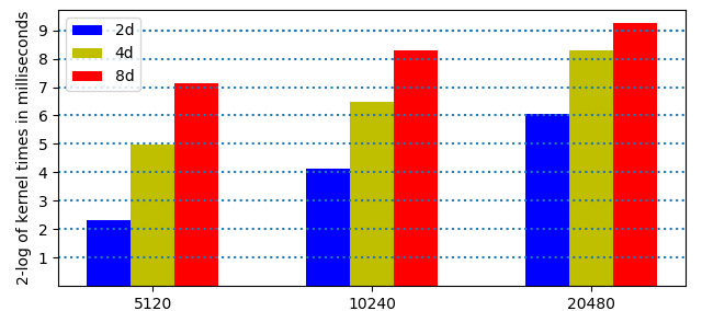
Fig. 94 2-logarithms of times on the V100 in 3 precisions
In Fig. 94, the heights of the bars are closer to each other in higher dimensions.
The V100 has 80 multiprocessors, its theoretical peak performance is 1.68 times that of the P100.
The value for \(N\) is fixed at 80, \(n\) runs from 32 to 256, see Fig. 95.
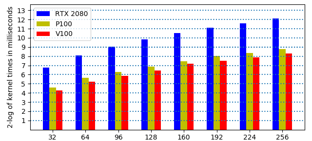
Fig. 95 kernel times in quad double precision on 3 GPUs
In Fig. 95, observe the heights of the bars as the dimensions double and the relative performance of the three different GPUs.
Considering \(20480 = 320 \times 64 = 160 \times 128 = 80 \times 256\), we run back substitution in quad double precision, for \(20480 = N \times n\), for three different combinations of \(N\) and \(n\), on the V100. The results are summarized in Table 24.
stage in Algorithm 1 |
\(320 \times 64\) |
\(160 \times 128\) |
\(80 \times 256\) |
|---|---|---|---|
invert diagonal tiles |
13.5 |
35.8 |
132.3 |
multiply with inverses |
49.0 |
47.5 |
64.3 |
back substitution |
84.6 |
91.7 |
112.3 |
time spent by kernels |
147.1 |
175.0 |
308.9 |
wall clock time |
2620.0 |
2265.0 |
2071.0 |
kernel time flops |
683.0 |
861.1 |
1136.1 |
wall clock flops |
38.3 |
66.5 |
169.5 |
The units of all times in Table 24 are milliseconds, flops unit is Gigaflops.
Bibliography
T.J. Dekker. A floating-point technique for extending the available precision. Numerische Mathematik, 18(3):224-242, 1971.
D. H. Heller. A survey of parallel algorithms in numerical linear algebra. SIAM Review, 20(4):740-777, 1978.
Y. Hida, X.S. Li, and D.H. Bailey. Algorithms for quad-double precision floating point arithmetic. In 15th IEEE Symposium on Computer Arithmetic, pages 155-162. IEEE, 2001. Software at <http://crd.lbl.gov/~dhbailey/mpdist>.
N. J. Higham. Stability of parallel triangular system solvers. SIAM J. Sci. Comput., 16(2):400-413, 1995.
M. Joldes, J.-M. Muller, V. Popescu, W. Tucker. CAMPARY: Cuda Multiple Precision Arithmetic Library and Applications. In Mathematical Software – ICMS 2016, the 5th International Conference on Mathematical Software, pages 232-240, Springer-Verlag, 2016.
M. Lu, B. He, and Q. Luo. Supporting extended precision on graphics processors. In A. Ailamaki and P.A. Boncz, editors, Proceedings of the Sixth International Workshop on Data Management on New Hardware (DaMoN 2010), June 7, 2010, Indianapolis, Indiana, pages 19-26, 2010. Software at <https://code.google.com/archive/p/gpuprec>.
W. Nasri and Z. Mahjoub. Optimal parallelization of a recursive algorithm for triangular matrix inversion on MIMD computers. Parallel Computing, 27:1767-1782, 2001.
J. Verschelde. Least squares on GPUs in multiple double precision. In The 2022 IEEE International Parallel and Distributed Processing Symposium Workshops (IPDPSW), pages 828-837. IEEE, 2022. Code at <https://github.com/janverschelde/PHCpack/src/GPU>.
D. Viswanath and L. N. Trefethen. Condition numbers of random triangular matrices. SIAM J. Matrix Anal. Appl., 19(2):564-581, 1998.
Exercises
Write a parallel solver with OpenMP to solve \(U {\bf x} = {\bf y}\).
Take for \(U\) a matrix with random numbers in \([0,1]\), compute \(\bf y\) so all components of \(\bf x\) equal one. Test the speedup of your program, for large enough values of \(n\) and a varying number of cores.
Describe a parallel solver for upper triangular systems \(U {\bf y} = {\bf b}\) for distributed memory computers. Write a prototype implementation using MPI and discuss its scalability.
Consider a tiled lower triangular system \(L {\bf x} = {\bf b}\).