Barriers for Synchronizations

For message passing, we distinguish between a linear, a tree, and a butterfly barrier, introducing the sendrecv in MPI. As an example of a data parallel algorithm, we describe the prefix sum algorithm. In the third subsection, Brent’s theorem is stated and applied to the parallel summation problem.

Synchronizing Computations

In synchronized computations, processors pass through a number of stages in an algorithm.

Definition of synchronization barrier

A synchronization barrier guarantees that no processor continues to the next stage until all processors have finished the current stage.

In the above definition, the processor stands for a process, thread, or task. Examples in distributed memory, shared memory, and accelerated parallel processing are

• Message passing defines MPI_Barrier(MPI_Comm comm).

• OpenMP has the #pragma omp barrier construct.

• CUDA provides the instruction __syncthreads().

A barrier has two phases. The arrival or trapping phase is followed by the departure or release phase. The manager maintains a counter: only when all workers have sent to the manager, does the manager send messages to all workers. Pseudo code for a linear barrier in a manager/worker model is shown below.

code for manager              code for worker

for i from 1 to p-1 do
    receive from i            send to manager
for i from 1 to p-1 do
    send to i                 receive from manager

The counter implementation of a barrier or linear barrier is effective but it takes \(O(p)\) steps. A schematic of the steps to synchronize 8 processes is shown in Fig. 96 for a linear and a tree barrier.

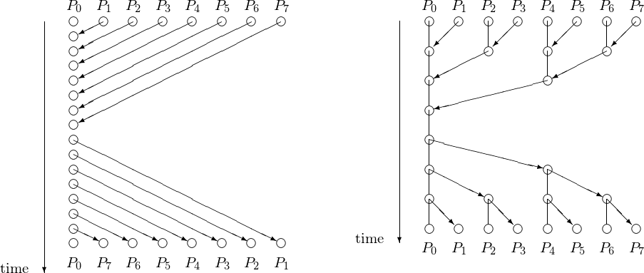
Fig. 96 A linear next to a tree barrier to synchronize 8 processes. For 8 processes, the linear barrier takes twice as many time steps as the tree barrier.

Implementing a tree barrier we write pseudo code for the trapping and the release phase, for \(p = 2^k\) (recall the fan in gather and the fan out scatter):

The trapping phase is defined below:

for i from k-1 down to 0 do
    for j from 2**i to 2**(i+1) do
        node j sends to node j - 2**i
        node j - 2**i receives from node j.

The release phase is defined below

for i from 0 to k-1 do
    for j from 0 to 2**i-1  do
        node j sends to j + 2**i
        node j + 2**i receives from node j.

Observe that two processes can synchronize in one step. We can generalize this into a tree barrier so there are no idle processes. This leads to a butterfly barrier shown in Fig. 97.

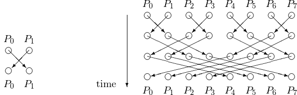
Fig. 97 Two processes can synchronize in one step as shown on the left. At the right is a schematic of the time steps for a tree barrier to synchronize 8 processes.

The algorithm for a butterfly barrier, for \(p = 2^k\), is described is pseudo code below.

for i from 0 to k-1 do
    s := 0
    for j from 0 to p-1 do
        if (j mod 2**(i+1) = 0) s := j
        node j sends to node ((j + 2**i) mod 2**(i+1)) + s
        node ((j + 2**i) mod 2^(i+1)) + s receives from node j

To avoid deadlock, ensuring that every send is matched with a corresponding receive, we can work with a sendrecv, as shown in Fig. 98.

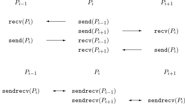
Fig. 98 The top picture is equivalent to the bottom picture.

The sendrecv in MPI has the following form:

MPI_Sendrecv(sendbuf,sendcount,sendtype,dest,sendtag,
             recvbuf,recvcount,recvtype,source,recvtag,comm,status)

where the parameters are in Table 25.

Table 25 Parameters of sendrecv in MPI.

parameter	description
sendbuf	initial address of send buffer
sendcount	number of elements in send buffer
sendtype	type of elements in send buffer
dest	rank of destination
sendtag	send tag
recvbuf	initial address of receive buffer
recvcount	number of elements in receive buffer
sendtype	type of elements in receive buffer
source	rank of source or MPI_ANY_SOURCE
recvtag	receive tag or MPI_ANY_TAG
comm	communicator
status	status object

We illustrate MPI_Sendrecv to synchronize two nodes. Processors 0 and 1 swap characters in a bidirectional data transfer.

$ mpirun -np 2 /tmp/use_sendrecv
Node 0 will send a to 1
Node 0 received b from 1
Node 1 will send b to 0
Node 1 received a from 0
$

with code below:

#include <stdio.h>
#include <mpi.h>

#define sendtag 100

int main ( int argc, char *argv[] )
{
   int i,j;
   MPI_Status status;

   MPI_Init(&argc,&argv);
   MPI_Comm_rank(MPI_COMM_WORLD,&i);

   char c = 'a' + (char)i; /* send buffer */
   printf("Node %d will send %c to %d\n",i,c,j);
   char d;                 /* receive buffer */

   MPI_Sendrecv(&c,1,MPI_CHAR,j,sendtag,&d,1,MPI_CHAR,MPI_ANY_SOURCE,
                MPI_ANY_TAG,MPI_COMM_WORLD,&status);

   printf("Node %d received %c from %d\n",i,d,j);
}

MPI_Finalize();
return 0;

The Prefix Sum Algorithm

A data parallel computation is a computation where the same operations are preformed on different data simultaneously. The benefits of data parallel computations is that they are easy to program, scale well, and are fit for SIMD computers. The problem we consider is to compute \(\displaystyle \sum_{i=0}^{n-1} a_i\) for \(n = p = 2^k\). This problem is related to the composite trapezoidal rule.

For \(n = 8\) and \(p = 8\), the prefix sum algorithm is illustrated in Fig. 99.

Fig. 99 The prefix sum for \(n = 8 = p\).

Pseudo code for the prefix sum algorithm for \(n = p = 2^k\) is below. Processor i executes:

s := 1
x := a[i]
for j from 0 to k-1 do
    if (j < p - s + 1) send x to processor i+s
    if (j > s-1) receive y from processor i-s
                 add y to x: x := x + y
    s := 2*s

The speedup: \(\displaystyle \frac{p}{\log_2(p)}\). Communication overhead: one send/recv in every step.

The prefix sum algorithm can be coded up in MPI as in the program below.

#include <stdio.h>
#include "mpi.h"
#define tag 100               /* tag for send/recv */

int main ( int argc, char *argv[] )
{
   int i,j,nb,b,s;
   MPI_Status status;
   const int p = 8;        /* run for 8 processors */

   MPI_Init(&argc,&argv);
   MPI_Comm_rank(MPI_COMM_WORLD,&i);

   nb = i+1;            /* node i holds number i+1 */
   s = 1;     /* shift s will double in every step */

   for(j=0; j<3; j++)              /* 3 stages, as log2(8) = 3 */
   {
      if(i < p - s)     /* every one sends, except last s ones */
         MPI_Send(&nb,1,MPI_INT,i+s,tag,MPI_COMM_WORLD);
      if(i >= s)     /* every one receives, except first s ones */
      {
         MPI_Recv(&b,1,MPI_INT,i-s,tag,MPI_COMM_WORLD,&status);
         nb += b;       /* add received value to current number */
      }
      MPI_Barrier(MPI_COMM_WORLD);  /* synchronize computations */
      if(i < s)
         printf("At step %d, node %d has number %d.\n",j+1,i,nb);
      else
         printf("At step %d, Node %d has number %d = %d + %d.\n",
                j+1,i,nb,nb-b,b);
   s *= 2;                               /* double the shift */
   }
   if(i == p-1) printf("The total sum is %d.\n",nb);

   MPI_Finalize();
   return 0;
}

Running the code prints the following to screen:

$ mpirun -np 8 /tmp/prefix_sum
At step 1, node 0 has number 1.
At step 1, Node 1 has number 3 = 2 + 1.
At step 1, Node 2 has number 5 = 3 + 2.
At step 1, Node 3 has number 7 = 4 + 3.
At step 1, Node 7 has number 15 = 8 + 7.
At step 1, Node 4 has number 9 = 5 + 4.
At step 1, Node 5 has number 11 = 6 + 5.
At step 1, Node 6 has number 13 = 7 + 6.
At step 2, node 0 has number 1.
At step 2, node 1 has number 3.
At step 2, Node 2 has number 6 = 5 + 1.
At step 2, Node 3 has number 10 = 7 + 3.
At step 2, Node 4 has number 14 = 9 + 5.
At step 2, Node 5 has number 18 = 11 + 7.
At step 2, Node 6 has number 22 = 13 + 9.
At step 2, Node 7 has number 26 = 15 + 11.
At step 3, node 0 has number 1.
At step 3, node 1 has number 3.
At step 3, node 2 has number 6.
At step 3, node 3 has number 10.
At step 3, Node 4 has number 15 = 14 + 1.
At step 3, Node 5 has number 21 = 18 + 3.
At step 3, Node 6 has number 28 = 22 + 6.
At step 3, Node 7 has number 36 = 26 + 10.
The total sum is 36.

Brent’s Theorem

PRAM stands for Parallel Random Access Machine The PRAM model is an idealized construct.

• It assumes any number of processors can access any items in memory instantly.

• An operation takes one unit time.

The PRAM model helps to derive bounds on the theoretical time of a parallel algorithm.

Brent’s theorem

Assume

1. a parallel computer where each processor can perform an arithmetic operation in unit time; and

2. the computer has exactly enough processors to exploit the maximum concurrency in an algorithm with \(N\) operations, such that \(T\) time steps suffice,

then a computer with \(P\) processors can perform the algorithm in time

\[T_P \leq T + \frac{N-T}{P},\]

where \(P\) is less than or equal to the number of processors needed to exploit the maximum concurrency in the algorithm.

As an application of Brent’s theorem, we look at parallel summation. Consider the sum of \(n\) numbers.

If \(n = 2^T\), then the PRAM can do the sum in \(T\) steps.

If the PRAM has \(P\) processors and \(P \leq n/2\), then

\[T_P \leq \lceil \log_2(n) \rceil + \frac{(n-1) - \log_2(n)}{P},\]

where \(T_P\) is the execution time with \(P\) processors.

Typically, the number of processors is fixed, and then we want to find the best size \(n\) of the problem so the theoretical bounds on the execution time are within reach.

Bibliography

1. R. P. Brent: The parallel evaluation of general arithmetic expressions. Journal of the ACM 12(2): 201-206, 1974.

2. John Gustafson: Brent’s Theorem. In Enclopedia of Parallel Computing, edited by David Padua, pages 182-185, Springer 2011.

3. W. Daniel Hillis and Guy L. Steele. Data Parallel Algorithms. Communications of the ACM, vol. 29, no. 12, pages 1170-1183, 1986.

Exercises

1. Does the hypercube topology support a butterfly barrier? If not, explain with an example. Otherwise, show that the hypercube topology has sufficiently many connections for a butterfly barrier.

2. Write code using MPI_sendrecv for a butterfly barrier. Show that your code works for \(p = 8\).

3. Rewrite prefix_sum.c using MPI_sendrecv.

4. Consider the composite trapezoidal rule for the approximation of \(\pi\) (see lecture 13), doubling the number of intervals in each step. Can you apply the prefix sum algorithm so that at the end, processor \(i\) holds the approximation for \(\pi\) with \(2^i\) intervals?