Introduction
In this first lecture we define supercomputing, speedup, and efficiency. Gustafson’s Law reevaluates Amdahl’s Law.
What is a Supercomputer?
Doing supercomputing means to use a supercomputer and is also called high performance computing.
Definition of Supercomputer
A supercomputer is a computing system (hardware, system & application software) that provides close to the best currently achievable sustained performance on demanding computational problems.
The current classification of supercomputers can be found at the TOP500 Supercomputer Sites.
A flop is a floating point operation. Performance is often measured in the number of flops per second. If two flops can be done per clock cycle, then a processor at 3GHz can theoretically perform 6 billion flops (6 gigaflops) per second. All computers in the top 10 achieve more than 1 petaflop per second.
Some system terms and architectures are listed below:
- core for a CPU: unit capable of executing a thread, for a GPU: a streaming multiprocessor.
- \({\rm R}_{\rm max}\) maximal performance achieved on the LINPACK benchmark (solving a dense linear system) for problem size \({\rm N}_{\rm max}\), measured in Gflop/s.
- \({\rm R}_{\rm peak}\) theoretical peak performance measured in Gflop/s.
- Power total power consumed by the system.
Concerning the types of architectures, we note the use of commodity leading edge microprocessors running at their maximal clock and power limits. Alternatively supercomputers use special processor chips running at less than maximal power to achieve high physical packaging densities. Thirdly, we observe mix of chip types and accelerators (GPUs).
Measuring Performance
The next definition links speedup and efficiency.
Definition of Speedup and Efficiency
By \(p\) we denote the number of processors.
Efficiency is another measure for parallel performance:
In the best case, we hope: \(S(p) = p\) and \(E(p) = 100\%\). If \(E = 50\%\), then on average processors are idle for half of the time.
While we hope for \(S(p) = p\), we may achieve \(S(p) > p\) and achieve superlinear speedup. Consider for example a sequential search in an unsorted list. A parallel search by \(p\) processors divides the list evenly in \(p\) sublists.
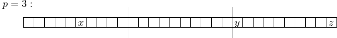
Fig. 1 A search illustrates superlinear speedup.
The sequential search time depends on position in list. The parallel search time depends on position in sublist. We obtain a huge speedup if the element we look for is for example the first element of the last sublist.
Amdahl’s and Gustafson’s Law
Consider a job that takes time \(t\) on one processor. Let \(R\) be the fraction of \(t\) that must be done sequentially, \(R \in [0,1]\). Consider Fig. 2.
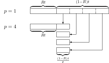
Fig. 2 Illustration of Amdahl’s Law.
We then calculate the speedup on \(p\) processors as
Amdahl’s Law (1967)
Let \(R\) be the fraction of the operations which cannot be done in parallel. The speedup with \(p\) processors is bounded by \(\displaystyle \frac{1}{R + \frac{1-R}{p}}\).
Corollary of Amdahl’s Law
\(\displaystyle S(p) \leq \frac{1}{R}\) as \(p \rightarrow \infty\).
Example of Amdahl’s Law
Suppose \(90\%\) of the operations in an algorithm can be executed in parallel. What is the best speedup with 8 processors? What is the best speedup with an unlimited amount of processors?
In contrast to Ahmdahl’s Law, we can start with the observation that many results obtained on supercomputers cannot be obtained one one processor. To derive the notion of scaled speedup, we start by considering a job that took time \(t\) on \(p\) processors. Let \(s\) be the fraction of \(t\) that is done sequentially.
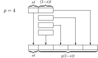
Fig. 3 Illustration of Gustafson’s Law.
The we computed the scaled speedup as follows:
We observe that the problem size scales with the number of processors!
Gustafson’s Law (1988)
If \(s\) is the fraction of serial operations in a parallel program run on \(p\) processors, then the scaled speedup is bounded by \(p + (1-p) s\).
Example of Gustafson’s Law
Suppose benchmarking reveals that \(5\%\) of time on a 64-processor machine is spent on one single processor (e.g.: root node working while all other processors are idle). Compute the scaled speedup.
More processing power often leads to better results, and we can achieve quality up. Below we list some examples.
- Finer granularity of a grid; e.g.: discretization of space and/or time in a differential equation.
- Greater confidence of estimates; e.g.: enlarged number of samples in a simulation.
- Compute with larger numbers (multiprecision arithmetic); e.g.: solve an ill-conditioned linear system.
If we can afford to spend the same amount of time on solving a problem then we can ask how much better we can solve the same problem with \(p\) processors? This leads to the notion of quality up.
\(Q(p)\) measures improvement in quality using \(p\) procesors, keeping the computational time fixed.
Bibliography
- S.G. Akl. Superlinear performance in real-time parallel computation. The Journal of Supercomputing, 29(1):89–111, 2004.
- J.L. Gustafson. Reevaluating Amdahl’s Law. Communications of the ACM, 31(5):532-533, 1988.
- P.M. Kogge and T.J. Dysart. Using the TOP500 to trace and project technology and architecture trends. In SC‘11 Proceedings of 2011 International Conference for High Performance Computing, Networking, Storage and Analysis. ACM 2011.
- B. Wilkinson and M. Allen. Parallel Programming. Techniques and Applications Using Networked Workstations and Parallel Computers. Prentice Hall, 2nd edition, 2005.
- J.M. Wing. Computational thinking. Communications of the ACM, 49(3):33-35, 2006.
Exercises
- How many processors whose clock speed runs at 3.0GHz does one need to build a supercomputer which achieves a theoretical peak performance of at least 4 Tera Flops? Justify your answer.
- Suppose we have a program where \(2\%\) of the operations must be executed sequentially. According to Amdahl’s law, what is the maximum speedup which can be achieved using 64 processors? Assuming we have an unlimited number of processors, what is the maximal speedup possible?
- Benchmarking of a program running on a 64-processor machine shows that \(2\%\) of the operations are done sequentially, i.e.: that \(2\%\) of the time only one single processor is working while the rest is idle. Use Gustafson’s law to compute the scaled speedup.