Classifications and Scalability

Parallel computers can be classified by instruction and data streams. Another distinction is between shared and distributed memory systems. We define clusters and the scalability of a problem. Network topologies apply both to hardware configurations and algorithms to transfer data.

Types of Parallel Computers

In 1966, Flynn introduced what is called the MIMD and SIMD classification:

• SISD: Single Instruction Single Data stream

  One single processor handles data sequentially. We use pipelining (e.g.: car assembly) to achieve parallelism.

• MISD: Multiple Instruction Single Data stream

  This is called systolic arrays and has been of little interest.

• SIMD: Single Instruction Multiple Data stream

  In graphics computing, one issues the same command for pixel matrix.

  One has vector and arrays processors for regular data structures.

• MIMD: Multiple Instruction Multiple Data stream

  This is the general purpose multiprocessor computer.

One model is SPMD: Single Program Multiple Data stream: All processors execute the same program. Branching in the code depends on the identification number of the processing node. Manager worker paradigm fits the SPMD model: manager (also called root) has identification zero; and workers are labeled \(1,2,\ldots,p-1\).

The distinction between shared and distributed memory parallel computers is illustrated with an example in Fig. 4.

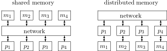
Fig. 4 A shared memory multicomputer has one single address space, accessible to every processor. In a distributed memory multicomputer, every processor has its own memory accessible via messages through that processor. Most nodes in a parallel computers have multiple cores.

Clusters and Scalability

Definition of Cluster

A cluster is an independent set of computers combined into a unified system through software and networking.

Beowulf clusters are scalable performance clusters based on commodity hardware, on a private network, with open source software.

Three factors drove the clustering revolution in computing. First is the availability of commodity hardware: choice of many vendors for processors, memory, hard drives, etc... Second, concerning networking, Ethernet is dominating commodity networking technology, supercomputers have specialized networks. The third factor consists of open source software infrastructure: Linux and MPI.

We next discuss scalability as it relates to message passing in clusters.

\[\mbox{total time} = \mbox{computation time} + \underbrace{\mbox{communication time}}_{\rm {\bf o~v~e~r~h~e~a~d}}\]

Because we want to reduce the overhead, the

\[\mbox{computation/communication ratio} = \frac{\mbox{computation time}}{\mbox{communication time}}\]

determines the scalability of a problem: The question is How well can we increase the problem size n, keeping p, the number of processors fixed? We desire that the order of overhead \(\ll\) order of computation, so ratio \(\rightarrow \infty\), Examples: \(O(\log_2(n)) < O(n) < O(n^2)\). One remedy is to overlap the communication with computation.

In a distributed shared memory computer: the memory is physically distributed with each processor; and each processor has access to all memory in single address space. The benefits are that message passing often not attractive to programmers; and while shared memory computers allow limited number of processors, distributed memory computers scale well. The disadvantage is that access to remote memory location causes delays and the programmer does not have control to remedy the delays.

Network Topologies

We distinguish between static connections and dynamic network topologies enabled by switches. Below is some terminology.

• bandwidth: number of bits transmitted per second

• on latency, we distinguish tree types:

  • message latency: time to send zero length message (or startup time),
  • network latency: time to make a message transfer the network,
  • communication latency: total time to send a message including software overhead and interface delays.

• diameter of network: minimum number of links between nodes that are farthest apart

• on bisecting the network:

  bisection width: number of links needed to cut network

  in two equal parts,

  bisection bandwidth: number of bits per second which can

  be sent from one half of network to the other half.

Connecting \(p\) nodes in complete graph is too expensive. Small examples of an array and ring topology are shown in Fig. 5. A matrix and torus of 16 nodes is shown in Fig. 6.

Fig. 5 An array and ring of 4 notes.

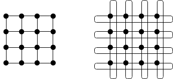
Fig. 6 A matrix and torus of 16 nodes.

A hypercube network is defined as follows. Two nodes are connected \(\Leftrightarrow\) their labels differ in exactly one bit. Simple examples are shown in Fig. 7.

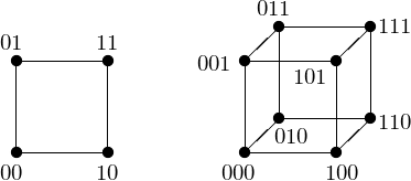
Fig. 7 Two special hypercubes: a square and cube.

e-cube or left-to-right routing: flip bits from left to right, e.g.: going from node 000 to 101 passes through 100. In a hypercube network with \(p\) nodes, the maximum number of flips is \(\log_2(p)\), and the number of connections is \(\ldots\)?

Consider a binary tree. The leaves in the tree are processors. The interior nodes in the tree are switches. This gives rise to a tree network, shown in Fig. 8.

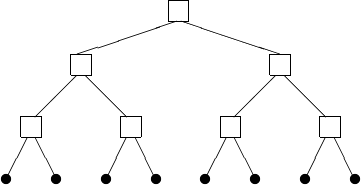
Fig. 8 A binary tree network.

Often the tree is fat: with an increasing number of links towards the root of the tree.

Dynamic network topologies are realized by switches. In a shared memory multicomputer, processors are usually connected to memory modules by a crossbar switch. An example, for \(p = 4\), is shown in Fig. 9.

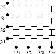
Fig. 9 Processors connected to memory modules via a crossbar switch.

A \(p\)-processor shared memory computer requires \(p^2\) switches. 2-by-2 switches are shown in Fig. 10.

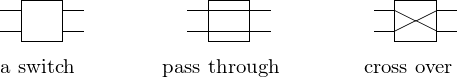
Fig. 10 2-by-2 swiches.

Changing from pass through to cross over configuration changes the connections between the computers in the network, see Fig. 11.

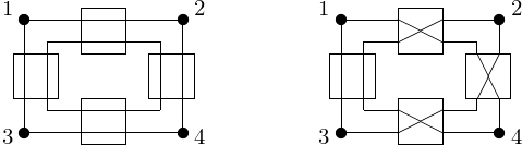
Fig. 11 Changing switches from pass through to cross over.

The rules in the routing algorithm in a multistage network are the following:

1. bit is zero: select upper output of switch; and
2. bit is one: select lower output of switch.

The first bit in the input determines the output of the first switch, the second bit in the input determines the output of the second switch. Fig. 12 shows a 2-stage network between 4 nodes.

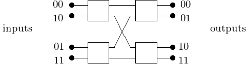
Fig. 12 A 2-stage network between 4 nodes.

The communication between 2 nodes using 2-by-2 switches causes blocking: other nodes are prevented from communicating. The number of switches for \(p\) processors equals \(\log_2(p) \times \frac{p}{2}\). Fig. 13 shows the application of circuit switching for \(p = 2^3\).

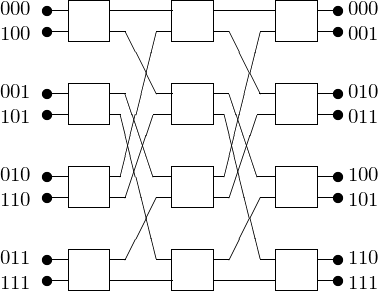
Fig. 13 A 3-stage Omega interconnection network.

We distinguish between circuit and packet switching. If all circuits are occupied, communication is blocked. Alternative solution: packet switching: message is broken in packets and sent through network. Problems to avoid:

• deadlock: Packets are blocked by other packets waiting to be forwarded. This occurs when the buffers are full with packets. Solution: avoid cycles using e-cube routing algorithm.
• livelock: a packet keeps circling the network and fails to find its destination.

The network in a typical cluster is shown in Fig. 14.

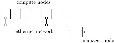
Fig. 14 A cluster connected via ethernet.

Modern workstations are good for software development and for running modest test cases to investigate scalability. We give two examples. HP workstation Z800 RedHat Linux: two 6-core Intel Xeon at 3.47Ghz, 24GB of internal memory, and 2 NVDIA Tesla C2050 general purpose graphic processing units. Microway whisperstation RedHat Linux: two 8-core Intel Xeon at 2.60Ghz, 128GB of internal memory, and 2 NVDIA Tesla K20C general purpose graphic processing units.

The Hardware Specs of the new UIC Condo cluster is at <http://rc.uic.edu/hardware-specs>:

• Two login nodes are for managing jobs and file system access.
• 160 nodes, each node has 16 cores, running at 2.60GHz, 20MB cache, 128GB RAM, 1TB storage.
• 40 nodes, each node has 20 cores, running at 2.50GHz, 20MB cache, 128GB RAM, 1TB storage.
• 3 large memory compute nodes, each with 32 cores having 1TB RAM giving 31.25GB per core. Total adds upto 96 cores and 3TB of RAM.
• Total adds up to 3,456 cores, 28TB RAM, and 203TB storage.
• 288TB fast scratch communicating with nodes over QDR infiniband.
• 1.14PB of raw persistent storage.

Bibliography

1. M.J. Flynn and K. W. Rudd. Parallel Architectures. ACM Computing Surveys 28(1): 67-69, 1996.
2. A. Grama, A. Gupta, G. Karypis, V. Kumar. Introduction to Parallel Computing. Pearson. Addison-Wesley. Second edition, 2003.
3. G.K. Thiruvathukal. Cluster Computing. Guest Editor’s Introduction. Computing in Science and Engineering 7(2): 11-13, 2005.
4. B. Wilkinson and M. Allen. Parallel Programming. Techniques and Applications Using Networked Workstations and Parallel Computers. Prentice Hall, 2nd edition, 2005.

Exercises

1. Derive a formula for the number of links in a hypercube with \(p = 2^k\) processors for some positive number \(k\).
2. Consider a network of 16 nodes, organized in a 4-by-4 mesh with connecting loops to give it the topology of a torus (or doughnut). Can you find a mapping of the nodes which give it the topology of a hypercube? If so, use 4 bits to assign labels to the nodes. If not, explain why.
3. We derived an Omega network for eight processors. Give an example of a configuration of the switches which is blocking, i.e.: a case for which the switch configurations prevent some nodes from communicating with each other.
4. Draw a multistage Omega interconnection network for \(p = 16\).