High Level Parallel Processing¶

In this lecture we give three examples of what could be considered high level parallel processing. First we see how we may accelerate matrix-matrix multiplication using the computer algebra system Maple. Then we explore the multiprocessing module in Python and finally we show how multitasking in the object-oriented language Ada is effective in writing parallel programs.

In high level parallel processing we can use an existing programming environment to obtain parallel implementations of algorithms. In this lecture we give examples of three fundamentally different programming tools to achieve parallelism: multi-processing (distributed memory), multi-threading (shared memory), and use of accelerators (general purpose graphics processing units).

There is some sense of subjectivity with the above description of what high level means. If unfamiliar with Maple, Python, or Ada, then the examples in this lecture may also seem too technical. What does count as high level is that we do not worry about technical issues as communication overhead, resource utilitization, synchronization, etc., but we ask only two questions. Is the parallel code correct? Does the parallel code run faster?

GPU computing with Maple¶

Maple is one of the big M’s in scientific software. UIC has a campus wide license: available in labs. Well documented and supported. Since version 15, Maple 15 enables GPU computing and we can accelerate a matrix-matrix multiplication.

Experiments done on HP workstation Z800 with NVDIA Tesla C2050 general purpose graphic processing unit. The images in Fig. 15 and Fig. 16 are two screen shots of Maple worksheets.

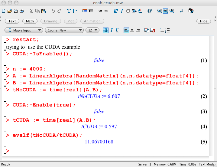
Fig. 15 First screen shot of a Maple worksheet.

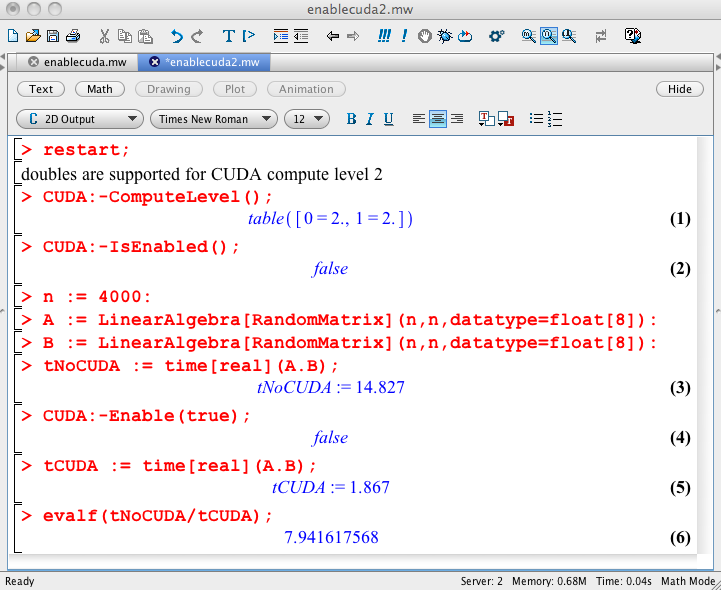
Fig. 16 Second screen shot of a Maple worksheet.

As example application of matrix-matrix application, we consider a Markov chain. A stochastic process is a sequence of events depending on chance. A Markov process is a stochastic process with (1) a finite set of possible outcomes; (2) the probability of the next outcome depends only on the previous outcome; and (3) all probabilities are constant over time. Realization: ${\bf x}^{(k+1)} = A {\bf x}^{(k)}$, for $k=0,1,\ldots$, where $A$ is an $n$-by-$n$ matrix of probabilities and the vector ${\bf x}$ represents the state of the process. The sequence ${\bf x}^{(k)}$ is a Markov chain. We are interested in the long term behaviour: ${\bf x}^{(k+1)} = A^{k+1} {\bf x}{(0)}$.

As an application of Markov chains, consider the following model: UIC has about 3,000 new incoming freshmen each Fall. The state of each student measures time till graduation. Counting historical passing grades in gatekeeper courses give probabilities to transition from one level to the next. Our Goal is to model time till graduation based on rates of passing grades.

Although the number of matrix-matrix products is relatively small, to study sensitivity and what-if scenarios, many runs are needed.

Multiprocessing in Python¶

Some advantages of the scripting language Python are: educational, good for novice programmers, modules for scientfic computing: NumPy, SciPy, SymPy. Sage, a free open source mathematics software system, uses Python to interface many free and open source software packages. Our example: $\displaystyle \int_0^1 \sqrt{1-x^2} dx = \frac{\pi}{4}$. We will use the Simpson rule (available in SciPy) as a relatively computational intensive example.

We develop our scripts in an interactive Python shell:

$ python
Python 2.6.1 (r261:67515, Jun 24 2010, 21:47:49)
[GCC 4.2.1 (Apple Inc. build 5646)] on darwin
Type "help", "copyright", "credits" or "license" for more information.
>>> from scipy.integrate import simps
>>> from scipy import sqrt, linspace, pi
>>> f = lambda x: sqrt(1-x**2)
>>> x = linspace(0,1,1000)
>>> y = f(x)
>>> I = simps(y,x)
>>> 4*I
3.1415703366671113

The script simpson4pi.py is below:

from scipy.integrate import simps
from scipy import sqrt, linspace, pi
f = lambda x: sqrt(1-x**2)
x = linspace(0,1,100); y = f(x)
I = 4*simps(y,x); print '10^2', I, abs(I - pi)
x = linspace(0,1,1000); y = f(x)
I = 4*simps(y,x); print '10^3', I, abs(I - pi)
x = linspace(0,1,10000); y = f(x)
I = 4*simps(y,x); print '10^4', I, abs(I - pi)
x = linspace(0,1,100000); y = f(x)
I = 4*simps(y,x); print '10^5', I, abs(I - pi)
x = linspace(0,1,1000000); y = f(x)
I = 4*simps(y,x); print '10^6', I, abs(I - pi)
x = linspace(0,1,10000000); y = f(x)
I = 4*simps(y,x); print '10^7', I, abs(I - pi)

To run the script simpson4pi.py, We type at the command prompt $:

$ python simpson4pi.py
10^2 3.14087636133 0.000716292255311
10^3 3.14157033667 2.23169226818e-05
10^4 3.1415919489 7.04691599296e-07
10^5 3.14159263131 2.2281084977e-08
10^6 3.14159265289 7.04557745479e-10
10^7 3.14159265357 2.22573071085e-11

The slow convergence makes that this is certainly not a very good way to approximate $\pi$, but it fits our purposes. We have a slow computationally intensive process that we want to run in parallel.

We measure the time it takes to run a script as follows. Saving the content of

from scipy.integrate import simps
from scipy import sqrt, linspace, pi
f = lambda x: sqrt(1-x**2)
x = linspace(0,1,10000000); y = f(x)
I = 4*simps(y,x)
print I, abs(I - pi)

into the script simpson4pi1.py, we use the unix time command.

$ time python simpson4pi1.py
3.14159265357 2.22573071085e-11

real    0m2.853s
user    0m1.894s
sys     0m0.956s

The real is the so-called wall clock time, user indicates the time spent by the processor and sys is the system time.

Python has a multiprocessing module. The script belows illustrates its use.

from multiprocessing import Process
import os
from time import sleep

def say_hello(name,t):
    """
    Process with name says hello.
    """
    print 'hello from', name
    print 'parent process :', os.getppid()
    print 'process id :', os.getpid()
    print name, 'sleeps', t, 'seconds'
    sleep(t)
    print name, 'wakes up'

pA = Process(target=say_hello, args = ('A',2,))
pB = Process(target=say_hello, args = ('B',1,))
pA.start(); pB.start()
print 'waiting for processes to wake up...'
pA.join(); pB.join()
print 'processes are done'

Running the script shows the following on screen:

$ python multiprocess.py
waiting for processes to wake up...
hello from A
parent process : 737
process id : 738
A sleeps 2 seconds
hello from B
parent process : 737
process id : 739
B sleeps 1 seconds
B wakes up
A wakes up
processes are done

Let us do numerical integration with multiple processes, with the script simpson4pi2.py listed below.

from multiprocessing import Process, Queue
from scipy import linspace, sqrt, pi
from scipy.integrate import simps

def call_simpson(fun, a,b,n,q):
    """
    Calls Simpson rule to integrate fun
    over [a,b] using n intervals.
    Adds the result to the queue q.
    """
    x = linspace(a, b, n)
    y = fun(x)
    I = simps(y, x)
    q.put(I)

def main():
    """
    The number of processes is given at the command line.
    """
    from sys import argv
    if len(argv) < 2:
        print 'Enter the number of processes at the command line.'
        return
    npr = int(argv[1])
    crc = lambda x: sqrt(1-x**2)
    nbr = 20000000
    nbrsam = nbr/npr
    intlen = 1.0/npr
    queues = [Queue() for _ in range(npr)]
    procs = []
    (left, right) = (0, intlen)
    for k in range(1, npr+1):
        procs.append(Process(target=call_simpson, \
            args = (crc, left, right, nbrsam, queues[k-1])))
        (left, right) = (right, right+intlen)
    for process in procs:
        process.start()
    for process in procs:
        process.join()
    app = 4*sum([q.get() for q in queues])
    print app, abs(app - pi)

To check for speedup we run the script as follows:

$ time python simpson4pi2.py 1
3.14159265358 8.01003707807e-12

real    0m2.184s
user    0m1.384s
sys     0m0.793s
$ time python simpson4pi2.py 2
3.14159265358 7.99982302624e-12

real    0m1.144s
user    0m1.382s
sys     0m0.727s
$

We have as speedup 2.184/1.144 = 1.909.

Tasking in Ada¶

Ada is a an object-oriented standardized language. Strong typing aims at detecting most errors during compile time. The tasking mechanism implements parallelism. The gnu-ada compiler produces code that maps tasks to threads. The main point is that shared-memory parallel programming can be done in a high level programming language as Ada.

The Simpson rule as an Ada function is shown below:

type double_float is digits 15;

function Simpson
  ( f : access function ( x : double_float )
        return double_float;
    a,b : double_float ) return double_float is

-- DESCRIPTION :
--   Applies the Simpson rule to approximate the
--   integral of f(x) over the interval [a,b].

  middle : constant double_float := (a+b)/2.0;
  length : constant double_float := b - a;

begin
  return length*(f(a) + 4.0*f(middle) + f(b))/6.0;
end Simpson;

Calling Simpson in a main program:

with Ada.Numerics.Generic_Elementary_Functions;

package Double_Elementary_Functions is
new Ada.Numerics.Generic_Elementary_Functions(double_float);

function circle ( x : double_float ) return double_float is

-- DESCRIPTION :
--   Returns the square root of 1 - x^2.

begin
  return Double_Elementary_Functions.SQRT(1.0 - x**2);
end circle;

v : double_float := Simpson(circle'access,0.0,1.0);

The composite Simpson rule is written as

function Recursive_Composite_Simpson
  ( f : access function ( x : double_float )
        return double_float;
    a,b : double_float; n : integer ) return double_float is

-- DESCRIPTION :
--   Returns the integral of f over [a,b] with n subintervals,
--   where n is a power of two for the recursive subdivisions.

  middle : double_float;

begin
  if n = 1 then
    return Simpson(f,a,b);
  else
    middle := (a + b)/2.0;
    return Recursive_Composite_Simpson(f,a,middle,n/2)
         + Recursive_Composite_Simpson(f,middle,b,n/2);
  end if;
end Recursive_Composite_Simpson;

The main procedure is

procedure Main is

  v : double_float;
  n : integer := 16;

begin
  for k in 1..7 loop
    v := 4.0*Recursive_Composite_Simpson
               (circle'access,0.0,1.0,n);
    double_float_io.put(v);
    text_io.put("  error :");
    double_float_io.put(abs(v-Ada.Numerics.Pi),2,2,3);
    text_io.put("  for n = "); integer_io.put(n,1);
    text_io.new_line;
    n := 16*n;
  end loop;
end Main;

Compiling and executing at the command line (with a makefile):

$ make simpson4pi
gnatmake simpson4pi.adb -o /tmp/simpson4pi
gcc -c simpson4pi.adb
gnatbind -x simpson4pi.ali
gnatlink simpson4pi.ali -o /tmp/simpson4pi

$ /tmp/simpson4pi
3.13905221789359E+00  error : 2.54E-03  for n = 16
3.14155300930713E+00  error : 3.96E-05  for n = 256
3.14159203419701E+00  error : 6.19E-07  for n = 4096
3.14159264391183E+00  error : 9.68E-09  for n = 65536
3.14159265343858E+00  error : 1.51E-10  for n = 1048576
3.14159265358743E+00  error : 2.36E-12  for n = 16777216
3.14159265358976E+00  error : 3.64E-14  for n = 268435456

We define a worker task as follows:

task type Worker
  ( name : integer;
    f : access function ( x : double_float )
        return double_float;
    a,b : access double_float; n : integer;
    v : access double_float );

task body Worker is

  w : access double_float := v;

begin
  text_io.put_line("worker" & integer'image(name)
                            & " will get busy ...");
  w.all := Recursive_Composite_Simpson(f,a.all,b.all,n);
  text_io.put_line("worker" & integer'image(name)
                            & " is done.");
end Worker;

Launching workers is done as

type double_float_array is
  array ( integer range <> ) of access double_float;

procedure Launch_Workers
  ( i,n,m : in integer; v : in double_float_array ) is

-- DESCRIPTION :
--   Recursive procedure to launch n workers,
--   starting at worker i, to apply the Simpson rule
--   with m subintervals.  The result of the i-th
--   worker is stored in location v(i).

  step : constant double_float := 1.0/double_float(n);
  start : constant double_float := double_float(i-1)*step;
  stop : constant double_float := start + step;
  a : access double_float := new double_float'(start);
  b : access double_float := new double_float'(stop);
  w : Worker(i,circle'access,a,b,m,v(i));

begin
  if i >= n then
    text_io.put_line("-> all" & integer'image(n)
                              & " have been launched");
  else
    text_io.put_line("-> launched " & integer'image(i));
    Launch_Workers(i+1,n,m,v);
  end if;
end Launch_Workers;

We get the number of tasks at the command line:

function Number_of_Tasks return integer is

-- DESCRIPTION :
--   The number of tasks is given at the command line.
--   Returns 1 if there are no command line arguments.

  count : constant integer
        := Ada.Command_Line.Argument_Count;

begin
  if count = 0 then
    return 1;
  else
    declare
      arg : constant string
          := Ada.Command_Line.Argument(1);
    begin
      return integer'value(arg);
    end;
  end if;
end Number_of_Tasks;

The main procedure is below:

procedure Main is

  nbworkers : constant integer := Number_of_Tasks;
  nbintervals : constant integer := (16**7)/nbworkers;
  results : double_float_array(1..nbworkers);
  sum : double_float := 0.0;

begin
  for i in results'range loop
    results(i) := new double_float'(0.0);
  end loop;
  Launch_Workers(1,nbworkers,nbintervals,results);
  for i in results'range loop
    sum := sum + results(i).all;
  end loop;
  double_float_io.put(4.0*sum); text_io.put(" error :");
  double_float_io.put(abs(4.0*sum-Ada.Numerics.pi));
  text_io.new_line;
end Main;

Times in seconds obtained as time /tmp/simpson4pitasking p for p = 1, 2, 4, 8, 16, and 32 on kepler.

Table 1 Running times with Ada Tasking.¶
p	real	user	sys	speedup
1	8.926	8.897	0.002	1.00
2	4.490	8.931	0.002	1.99
4	2.318	9.116	0.002	3.85
8	1.204	9.410	0.003	7.41
16	0.966	12.332	0.003	9.24
32	0.792	14.561	0.009	11.27

Speedups are computed as $\displaystyle \frac{\mbox{real time with p = 1}} {\mbox{real time with p tasks}}$.

Performance Monitoring¶

perfmon2 is a hardware-based performance monitoring interface for the Linux kernel. To monitor the performance of a program, with the gathering of performance counter statistics, type

$ perf stat program

at the command prompt. To get help, type perf help. For help on perf stat, type perf stat help.

To count flops, we can select an event we want to monitor.

On the Intel Sandy Bridge processor, the codes for double operations are

0x530110 for FP_COMP_OPS_EXE:SSE_FP_PACKED_DOUBLE, and
0x538010 for FP_COMP_OPS_EXE:SSE_SCALAR_DOUBLE.

To count the number of double operations, we do

$ perf stat -e r538010 -e r530110 /tmp/simpson4pitasking 1

and the output contains

Performance counter stats for '/tmp/simpson4pitasking 1':

    4,932,758,276 r538010
    3,221,321,361 r530110

       9.116025034 seconds time elapsed

Exercises¶

For the Matrix-Matrix Multiplication of Maple with CUDA enabled investigate the importance of the size dimension $n$ to achieve a good speedup. Experiment with values for $n \leq 4000$.

For which values of $n$ does the speedup drop to 2?
Write a Maple worksheet to generate matrices of probabilities for use in a Markov chain and compute at least 100 elements in the chain. For a large enough dimension, compare the elapsed time with and without CUDA enabled. To time code segments in a Maple worksheet, place the code segment between

start := time() and stop := time() statements.

The time spent on the code segment is then the difference between stop and start.
A Monte Carlo method to estimate $\pi/4$ generates random tuples $(x,y)$, with $x$ and $y$ uniformly distributed in $[0,1]$. The ratio of the number of tuples inside the unit circle over the total number of samples approximates $\pi/4$.
```
>>> from random import uniform as u
>>> X = [u(0,1) for i in xrange(1000)]
>>> Y = [u(0,1) for i in xrange(1000)]
>>> Z = zip(X,Y)
>>> F = filter(lambda t: t[0]**2 + t[1]**2 <= 1, Z)
>>> len(F)/250.0
3.1440000000000001
```
Use the multiprocessing module to write a parallel version, letting processes take samples independently. Compute the speedup.
Compute the theoretical peak performance (expressed in giga or teraflops) of the two Intel Xeons E5-2670 in kepler.math.uic.edu. Justify your calculation.

High Level Parallel Processing¶

GPU computing with Maple¶

Multiprocessing in Python¶

Tasking in Ada¶

Performance Monitoring¶

Exercises¶

Table Of Contents

Previous topic

Next topic

This Page