Pleasingly Parallel Computations
Monte Carlo simulations are an example of a computation for which a parallel computation requires a constant amount of communication. In particular, at the start of the computations, the manager node gives every worker node a seed for its random numbers. At the end of the computations, the workers send their simulation result to the manager node. Between start and end, no communication occurred and we may expect an optimal speedup. This type of computation is called a pleasingly parallel computation.
Ideal Parallel Computations
Suppose we have a disconnected computation graph for 4 processes as in Fig. 20.
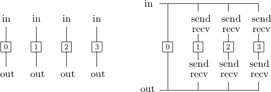
Fig. 20 One manager node distributes input data to the compute nodes and collects results from the compute nodes.
Even if the work load is well balanced and all nodes terminate at the same time, we still need to collect the results from each node. Without communication overhead, we hope for an optimal speedup.
Some examples of parallel computations without communication overhead are
- Geometric transformations of images (section 3.2.1 in textbook): Given an n-by-n matrix of pixels with RGB color encodings, the communication overhead is \(O(n^2)\). The cost of a transformation is at most \(O(n^2)\). While good for parallel computing, this is not good for message passing on distributed memory!
- The computation of the Mandelbrot set: Every pixel in the set may require up to 255 iterations. Pixels are computed independently from each other.
- Monte Carlo simulations: Every processor generates a different sequence of random samples and process samples independently.
In this lecture we elaborate on the third example.
Monte Carlo Simulations
We count successes of simulated experiments. We simulate by
- repeatedly drawing samples along a distribution;
- counting the number of successful samples.
By the law of large numbers, the average of the observed successes converges to the expected value or mean, as the number of experiments increases.
Estimating \(\pi\), the area of the unit disk as \(\displaystyle \int_0^1 \sqrt{1-x^2} dx = \frac{\pi}{4}\). Generating random uniformly distributed points with coordinates \((x,y) \in [0,+1] \times [0,+1]\), We count a success when \(x^2 + y^2 \leq 1\).
SPRNG: scalable pseudorandom number generator
We only have pseudorandom numbers as true random numbers do not exist on a computer... A multiplicative congruential generator is determined by multiplier a, additive constant c, and a modulus m:
Assumed: the pooled results of p processors running p copies of a Monte Carlo calculation achieves variance p times smaller.
However, this assumption is true only if the results on each processor are statistically independent. Some problems are that the choice of the seed determines the period, and with repeating sequences, we have lattice effects. The SPRNG: Scalable PseudoRandom Number Generators library is designed to support parallel Monte Carlo applications. A simple use is illustrated below:
#include <stdio.h>

#define SIMPLE_SPRNG /* simple interface */
#include "sprng.h"

int main ( void )
{
   printf("hello SPRNG...\n");
   double r = sprng();
   printf("a random double: %.15lf\n",r);
   return 0;
}
Because g++ (the gcc c++ compiler) was used to build SPRNG, the makefile is as follows.
sprng_hello:
        g++ -I/usr/local/include/sprng sprng_hello.c -lsprng \
            -o /tmp/sprng_hello
To see a different random double with each run of the program, we generate a new seed, as follows:
#include <stdio.h>
#define SIMPLE_SPRNG
#include "sprng.h"

int main ( void )
{
   printf("SPRNG generates new seed...\n");
   /* make new seed each time program is run   */
   int seed = make_sprng_seed();
   printf("the seed : %d\n", seed);
   /* initialize the stream */
   init_sprng(seed, 0, SPRNG_DEFAULT);
   double r = sprng();
   printf("a random double: %.15f\n", r);
   return 0;
}
Consider the estimation of \(\pi\) with SPRNG and MPI.
The progam sprng_estpi.c is below.
#include <stdio.h>
#include <math.h>
#define SIMPLE_SPRNG
#include "sprng.h"
#define PI 3.14159265358979

int main(void)
{
   printf("basic estimation of Pi with SPRNG...\n");
   int seed = make_sprng_seed();
   init_sprng(seed, 0, SPRNG_DEFAULT);

   printf("Give the number of samples : ");
   int n; scanf("%d", &n);

   int i, cnt=0;
   for(i=0; i<n; i++)
   {
      double x = sprng();
      double y = sprng();
      double z = x*x + y*y;
      if(z <= 1.0) cnt++;
   }
   double estimate = (4.0*cnt)/n;
   printf("estimate for Pi : %.15f", estimate);
   printf("  error : %.3e\n", fabs(estimate-PI));

   return 0;
}
And some runs:
$ /tmp/sprng_estpi
basic estimation of Pi with SPRNG...
Give the number of samples : 100
estimate for Pi : 3.200000000000000  error : 5.841e-02
$ /tmp/sprng_estpi
basic estimation of Pi with SPRNG...
Give the number of samples : 10000
estimate for Pi : 3.131200000000000  error : 1.039e-02
$ /tmp/sprng_estpi
basic estimation of Pi with SPRNG...
Give the number of samples : 10000
estimate for Pi : 3.143600000000000  error : 2.007e-03
$ /tmp/sprng_estpi
basic estimation of Pi with SPRNG...
Give the number of samples : 1000000
estimate for Pi : 3.140704000000000  error : 8.887e-04
Using MPI, we run the program sprng_estpi_mpi.c:
#include <stdio.h>
#include <math.h>
#define SIMPLE_SPRNG
#include "sprng.h"
#define PI 3.14159265358979
#include <mpi.h>

double estimate_pi ( int i, int n );
/* Estimation of pi by process i,
 * using n samples. */

int main ( int argc, char *argv[] )
{
   int id,np;

   MPI_Init(&argc,&argv);
   MPI_Comm_size(MPI_COMM_WORLD,&np);
   MPI_Comm_rank(MPI_COMM_WORLD,&id);

   int n;
   if(id == 0)
   {
      printf("Reading the number of samples...\n");
      scanf("%d",&n);
   }
   MPI_Bcast(&n,1,MPI_INT,0,MPI_COMM_WORLD);

   double est4pi = estimate_pi(id, n);
   double sum = 0.0;
   MPI_Reduce(&est4pi,&sum,1,MPI_DOUBLE,MPI_SUM,0,MPI_COMM_WORLD);
   if(id == 0)
   {
      est4pi = sum/np;
      printf("Estimate for Pi : %.15lf",est4pi);
      printf("  error : %.3e\n",fabs(est4pi-PI));
   }
   MPI_Finalize();
   return 0;
}
MPI_Reduce is a collective communication function to reduce
data gathered using some operations, e.g.: addition.
The syntax and arguments are in Table 6.
The predefined reduction operation op we use is MPI_SUM.
| MPI_REDUCE(sendbuf,recvbuf,count,datatype, op,root,comm) | |
|---|---|
| sendbuf | address of send buffer |
| recvbuf | address of receive buffer |
| count | number of elements in send buffer |
| datatype | data type of elements in send buffer |
| op | reduce operation |
| root | rank of root process |
| comm | communicator |
The estimate function we use in sprng_estpi_mpi.c is below:
double estimate_pi ( int i, int n )
{
   int seed = make_sprng_seed();
   init_sprng(seed, 0, SPRNG_DEFAULT);

   int j,cnt=0;
   for(j=0; j<n; j++)
   {
      double x = sprng();
      double y = sprng();
      double z = x*x + y*y;
      if(z <= 1.0) cnt++;
   }
   double estimate = (4.0*cnt)/n;
   printf("Node %d estimate for Pi : %.15f",i,estimate);
   printf("  error : %.3e\n",fabs(estimate-PI));

   return estimate;
}
Because g++ (the gcc C++ compiler) was used to build SPRNG,
we must compile the code with mpic++.
Therefore, the makefile contains the following lines:
sprng_estpi_mpi:
        mpic++ -I/usr/local/include/sprng \
               sprng_estpi_mpi.c -lsprng \
               -o /tmp/sprng_estpi_mpi
We end this section with the Mean Time Between Failures (MTBF) problem. The Mean Time Between Failures (MTBF) problem asks for the expected life span of a product made of components. Every component is critical. The multi-component product fails as soon as one of its components fails. For every component we assume that the life span follows a known normal distribution, given by \(\mu\) and \(\sigma\). For example, consider 3 components with respective means 11, 12, 13 and corresponding standard deviations 1, 2, 3. Running 100,000 simulations, we compute the average life span of the composite product.
If \(f_i(t)\) is the cumulative distribution function of the i-th component, then we estimate the triple integral:
We need to implement the normal distribution, as specified below.
int normal ( double *x, double *y );
/*
 * DESCRIPTION :
 *   Generates two independent normally distributed
 *   variables x and y, along Algorithm P (Knuth Vol 2),
 *   the polar method is due to Box and Muller.
 *
 * ON ENTRY :
 *   x,y     two independent random variables,
 *           uniformly distributed in [0,1].
 *
 * ON RETURN : fail = normal(&x,&y)
 *   fail    if 1, then x and y are outside the unit disk,
 *           if 0, then x and y are inside the unit disk;
 *   x,y     independent normally distributed variables. */
The function normal can be defined as
int normal ( double *x, double *y )
{
   double s;

   *x = 2.0*(*x) - 1.0;
   *y = 2.0*(*y) - 1.0;
   s = (*x)*(*x) + (*y)*(*y);

   if(s >= 1.0)
      return 1;
   else
   {
      double ln_s = log(s);
      double rt_s = sqrt(-2.0*ln_s/s);
      *x = (*x)*rt_s;
      *y = (*y)*rt_s;
      return 0;
   }
}
To test the function normal, we proceed as follows.
For the generated numbers,
we compute the average \(\mu\)
and standard deviation \(\sigma\).
We count how many samples are
in \([\mu - \sigma, \mu + \sigma]\).
$ /tmp/sprng_normal
normal variables with SPRNG ...
a normal random variable : 0.645521197140996
a normal random variable : 0.351776102906080
give number of samples : 1000000
mu = 0.000586448667516, sigma = 1.001564397361179
ratio of #samples in [-1.00,1.00] : 0.6822
generated 1572576 normal random numbers
To compile, we may need to link with the math library -lm.
The header (specification) of the function is
double map_to_normal ( double mu, double sigma, double x );
/*
 * DESCRIPTION :
 *   Given a normally distributed number x with mean 0 and
 *   standard deviation 1, returns a normally distributed
 *   number y with mean mu and standard deviation sigma. */
The C code (implementation) of the function is
double map_to_normal ( double mu, double sigma, double x )
{
   return mu + sigma*x;
}
Running sprng_mtbf gives
$ /tmp/sprng_mtbf
MTBF problem with SPRNG ...
Give number of components : 3
average life span for part 0 ? 11
standard deviation for part 0 ? 1
average life span for part 1 ? 12
standard deviation for part 1 ? 2
average life span for part 2 ? 13
standard deviation for part 2 ? 3
mu[0] = 11.000  sigma[0] = 1.000
mu[1] = 12.000  sigma[1] = 2.000
mu[2] = 13.000  sigma[2] = 3.000
Give number of simulations : 100000
expected life span : 10.115057028769346
The header of the mtbf function is below
#include <stdio.h>
#include <stdlib.h>
#include <math.h>
#define SIMPLE_SPRNG
#include "sprng.h"

double mtbf ( int n, int m, double *mu, double *sigma );
/*
 * DESCRIPTION :
 *   Returns the expected life span of a composite product
 *   of m parts, where part i has expected life span mu[i],
 *   with standard deviation sigma[i],
 *   using n simulations. */
The mtbf function is implemented as
double mtbf ( int n, int m, double *mu, double *sigma )
{
   int i,cnt=0;
   double s[n+1];
   do
   {
      normald(mu[0],sigma[0],&s[cnt],&s[cnt+1]);
      for(i=1; i<m; i++)
      {
         double x,y;
         normald(mu[i],sigma[i],&x,&y);
         s[cnt] = min(s[cnt],x);
         s[cnt+1] = min(s[cnt+1],y);
      }
      cnt = cnt + 2;
   } while (cnt < n);

   double sum = 0.0;
   for(i=0; i<cnt; i++) sum = sum + s[i];
   return sum/cnt;
}
Bibliography
- S.L. Anderson. Random number generators on vector supercomputers and other advanced architectures. SIAM Review 32(2): 221–251, 1990.
- D.E. Knuth. The Art of Computer Programming. Volume 2. Seminumerical Algorithms. Third Edition. Addison-Wesley, 1997. Chapter Three.
- M. Mascagni and A. Srinivasan. Algorithm 806: SPRNG: a scalable library for pseudorandom number generation. ACM Transactions on Mathematical Software 26(3): 436–461, 2000.
Exercises
- Consider the code for the estimation of \(\pi\). For a fixed choice of the seed, examine the relationship between the error \(\epsilon\) and the number of samples \(n\). Make a plot relating \(n\) to \(-\log_{10}(\epsilon)\), for sufficiently many experiments for different values of \(n\) so the trend becomes clear.
- Consider the MPI code for the estimation of \(\pi\). Fix the seeds so you can experimentally demonstrate the speedup. Execute the code for \(p = 2, 4\), and 8 compute nodes.
- Write a parallel version with MPI of
sprng_mtbf.c. Verify the correctness by comparison with a sequential run.