Load Balancing

We distinguish between static and dynamic load balancing, using the computation of the Mandelbrot set as an example. For dynamic load balancing, we encounter the need for nonblocking communications. To check for incoming messages, we use MPI_Iprobe.

the Mandelbrot set

We consider computing the Mandelbrot set, shown in Fig. 21 as a grayscale plot.

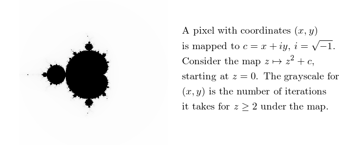
Fig. 21 The Mandelbrot set.

The number \(n\) of iterations ranges from 0 to 255. The grayscales are plotted in reverse, as \(255 - n\). Grayscales for different pixels are calculated independently. The prototype and definition of the function iterate is in the code below. We call iterate for all pixels (x, y), for x and y ranging over all rows and columns of a pixel matrix. In our plot we compute 5,000 rows and 5,000 columns.

int iterate ( double x, double y );
/*
 * Returns the number of iterations for z^2 + c
 * to grow larger than 2, for c = x + i*y,
 * where i = sqrt(-1), starting at z = 0. */

int iterate ( double x, double y )
{
   double wx,wy,v,xx;
   int k = 0;

   wx = 0.0; wy = 0.0; v = 0.0;
   while ((v < 4) && (k++ < 254))
   {
      xx = wx*wx - wy*wy;
      wy = 2.0*wx*wy;
      wx = xx + x;
      wy = wy + y;
      v = wx*wx + wy*wy;
   }
   return k;
}

In the code for iterate we count 6 multiplications on doubles, 3 additions and 1 subtraction. On a Mac OS X laptop 2.26 Ghz Intel Core 2 Duo, for a 5,000-by-5,000 matrix of pixels:

$ time /tmp/mandelbrot
Total number of iterations : 682940922

real    0m15.675s
user    0m14.914s
sys     0m0.163s

The program performed \(682,940,922 \times 10\) flops in 15 seconds or 455,293,948 flops per second. Turning on full optimization and the time drops from 15 to 9 seconds. After compilation with -O3, the program performed 758,823,246 flops per second.

$ make mandelbrot_opt
gcc -O3 -o /tmp/mandelbrot_opt mandelbrot.c

$ time /tmp/mandelbrot_opt
Total number of iterations : 682940922

real    0m9.846s
user    0m9.093s
sys     0m0.163s

The input parameters of the program define the intervals \([a,b]\) for \(x\) and \([c,d]\) for \(y\), as \((x,y) \in [a,b] \times [c,d]\), e.g.: \([a,b] = [-2,+2] = [c,d]\); The number \(n\) of rows (and columns) in pixel matrix determines the resolution of the image and the spacing between points: \(\delta x = (b-a)/(n-1)\), \(\delta y = (d-c)/(n-1)\). The output is a postscript file, which is a standard format, direct to print or view, and allows for batch processing in an environment without visualization capabilities.

Static Work Load Assignment

Static work load assignment means that the decision which pixels are computed by which processor is fixed in advance (before the execution of the program) by some algorithm. For the granularity in the communcation, we have two extremes:

1. Matrix of grayscales is divided up into p equal parts and each processor computes part of the matrix. For example: 5,000 rows among 5 processors, each processor takes 1,000 rows. The communication happens after all calculations are done, at the end all processors send their big submatrix to root node.
2. Matrix of grayscales is distributed pixel-by-pixel. Entry \((i,j)\) of the n-by-n matrix is computed by processor with label \(( i \times n + j ) ~{\rm mod}~ p\). The communication is completely interlaced with all computation.

In choosing the granularity between the two extremes:

1. Problem with all communication at end: Total cost = computational cost + communication cost. The communication cost is not interlaced with the computation.
2. Problem with pixel-by-pixel distribution: To compute the grayscale of one pixel requires at most 255 iterations, but may finish much sooner. Even in the most expensive case, processors may be mostly busy handling send/recv operations.

As compromise between the two extremes, we distribute the work load along the rows. Row \(i\) is computed by node \(1 + (i ~{\rm mod}~ (p-1))\). THe root node 0 distributes row indices and collects the computed rows.

Static work load assignment with MPI

Consider a manager/worker algorithm for static load assignment: Given \(n\) jobs to be completed by \(p\) processors, \(n \gg p\). Processor 0 is in charge of

1. distributing the jobs among the \(p-1\) compute nodes; and
2. collecting the results from the \(p-1\) compute nodes.

Assuming \(n\) is a multiple of \(p-1\), let \(k = n/(p-1)\).

The manager executes the following algorithm:

for i from 1 to k do
    for j from 1 to p-1 do
        send the next job to compute node j;
    for j from 1 to p-1 do
        receive result from compute node j.

The run of an example program is illustrated by what is printed on screen:

$ mpirun -np 3 /tmp/static_loaddist
reading the #jobs per compute node...
1
sending 0 to 1
sending 1 to 2
node 1 received 0
-> 1 computes b
node 1 sends b
node 2 received 1
-> 2 computes c
node 2 sends c
received b from 1
received c from 2
sending -1 to 1
sending -1 to 2
The result : bc
node 2 received -1
node 1 received -1
$

The main program is below, followed by the code for the worker and for the manager.

int main ( int argc, char *argv[] )
{
   int i,p;
   MPI_Init(&argc,&argv);
   MPI_Comm_size(MPI_COMM_WORLD,&p);
   MPI_Comm_rank(MPI_COMM_WORLD,&i);
   if(i != 0)
      worker(i);
   else
   {
      printf("reading the #jobs per compute node...\n");
      int nbjobs; scanf("%d",&nbjobs);
      manager(p,nbjobs*(p-1));
   }
   MPI_Finalize();
   return 0;
}

Following is the code for each worker.

int worker ( int i )
{
   int myjob;
   MPI_Status status;
   do
   {
      MPI_Recv(&myjob,1,MPI_INT,0,tag,
               MPI_COMM_WORLD,&status);
      if(v == 1) printf("node %d received %d\n",i,myjob);
      if(myjob == -1) break;
      char c = 'a' + ((char)i);
      if(v == 1) printf("-> %d computes %c\n",i,c);
      if(v == 1) printf("node %d sends %c\n",i,c);
      MPI_Send(&c,1,MPI_CHAR,0,tag,MPI_COMM_WORLD);
   }
   while(myjob != -1);
   return 0;
}

Following is the code for the manager.

int manager ( int p, int n )
{
   char result[n+1];
   int job = -1;
   int j;
   do
   {
      for(j=1; j<p; j++) /* distribute jobs */
      {
         if(++job >= n) break;
         int d = 1 + (job % (p-1));
         if(v == 1) printf("sending %d to %d\n",job,d);
         MPI_Send(&job,1,MPI_INT,d,tag,MPI_COMM_WORLD);
      }
      if(job >= n) break;
      for(j=1; j<p; j++) /* collect results */
      {
         char c;
         MPI_Status status;
         MPI_Recv(&c,1,MPI_CHAR,j,tag,MPI_COMM_WORLD,&status);
         if(v == 1) printf("received %c from %d\n",c,j);
         result[job-p+1+j] = c;
      }
   } while (job < n);

   job = -1;
   for(j=1; j < p; j++)  /* termination signal is -1 */
   {
      if(v==1) printf("sending -1 to %d\n",j);
      MPI_Send(&job,1,MPI_INT,j,tag,MPI_COMM_WORLD);
   }
   result[n] = '\0';
   printf("The result : %s\n",result);
   return 0;
}

Dynamic Work Load Balancing

Consider scheduling 8 jobs on 2 processors, as in Fig. 22.

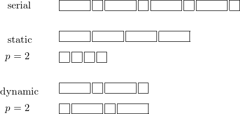
Fig. 22 Scheduling 8 jobs on 2 processors. In a worst case scenario, with static job scheduling, all the long jobs end up at one processor, while the short ones at the other, creating an uneven work load.

In scheduling \(n\) jobs on \(p\) processors, \(n \gg p\), node 0 manages the job queue, nodes 1 to \(p-1\) are compute nodes. The manager executes the following algorithm:

for j from 1 to p-1 do
    send job j-1 to compute node j;
while not all jobs are done do
    if a node is done with a job then
        collect result from node;
        if there is still a job left to do then
            send next job to node;
        else send termination signal.

To check for incoming messages, the nonblocking (or Immediate) MPI command is explained in Table 7.

Table 7 Syntax and arguments of MPI_Iprobe.

MPI_Iprobe(source,tag,comm,flag,status)
source	rank of source or MPI_ANY_SOURCE
tag	message tag or MPI_ANY_TAG
comm	communicator
flag	address of logical variable
status	status object

If flag is true on return, then status contains the rank of the source of the message and can be received. The manager starts with distributing the first \(p-1\) jobs, as shown below.

int manager ( int p, int n )
{
   char result[n+1];
   int j;

   for(j=1; j<p; j++) /* distribute first jobs */
   {
      if(v == 1) printf("sending %d to %d\n",j-1,j);
      MPI_Send(&j,1,MPI_INT,j,tag,MPI_COMM_WORLD);
   }
   int done = 0;
   int jobcount = p-1; /* number of jobs distributed */
   do                  /* probe for results */
   {
      int flag;
      MPI_Status status;
      MPI_Iprobe(MPI_ANY_SOURCE,MPI_ANY_TAG,
                 MPI_COMM_WORLD,&flag,&status);
      if(flag == 1)
      {              /* collect result */
         char c;
         j = status.MPI_SOURCE;
         if(v == 1) printf("received message from %d\n",j);
         MPI_Recv(&c,1,MPI_CHAR,j,tag,MPI_COMM_WORLD,&status);
         if(v == 1) printf("received %c from %d\n",c,j);
         result[done++] = c;
         if(v == 1) printf("#jobs done : %d\n",done);
         if(jobcount < n) /* send the next job */
         {
            if(v == 1) printf("sending %d to %d\n",jobcount,j);
            jobcount = jobcount + 1;
            MPI_Send(&jobcount,1,MPI_INT,j,tag,MPI_COMM_WORLD);
         }
         else  /* send -1 to signal termination */
         {
            if(v == 1) printf("sending -1 to %d\n",j);
            flag = -1;
            MPI_Send(&flag,1,MPI_INT,j,tag,MPI_COMM_WORLD);
         }
      }
   } while (done < n);
   result[done] = '\0';
   printf("The result : %s\n",result);
   return 0;
}

The code for the worker is the same as in the static work load distribution, see the function worker above. To make the simulation of the dynamic load balancing more realistic, the code for the worker could be modified with a call to the sleep function with as argument a random number of seconds.

Bibliography

1. George Cybenko. Dynamic Load Balancing for Distributed Memory Processors. Journal of Parallel and Distributed Computing 7, 279-301, 1989.

Exercises

1. Apply the manager/worker algorithm for static load assignment to the computation of the Mandelbrot set. What is the speedup for 2, 4, and 8 compute nodes? To examine the work load of every worker, use an array to store the total number of iterations computed by every worker.
2. Apply the manager/worker algorithm for dynamic load balancing to the computation of the Mandelbrot set. What is the speedup for 2, 4, and 8 compute nodes? To examine the work load of every worker, use an array to store the total number of iterations computed by every worker.
3. Compare the performance of static load assignment with dynamic load balancing for the Mandelbrot set. Compare both the speedups and the work loads for every worker.