Solving Triangular Systems
We apply a type 3 pipeline to solve a triangular linear system. Rewriting the formulas for the forward substitution we arrive at an implementation for shared memory computers with OpenMP. For accurate results, we compute with quad double arithmetic.
Forward Substitution Formulas
The LU factorization of a matrix \(A\) reduces the solving of a linear system to solving two triangular systems. To solve an n-dimensional linear system \(A {\bf x} = {\bf b}\) we factor A as a product of two triangular matrices, \(A = L U\):
- \(L\) is lower triangular, \(L = [\ell_{i,j}]\), \(\ell_{i,j} = 0\) if \(j > i\) and \(\ell_{i,i} = 1\).
- \(U\) is upper triangular \(U = [u_{i,j}]\), \(u_{i,j} = 0\) if \(i > j\).
Solving \(A {\bf x} = {\bf b}\) is equivalent to solving \(L(U {\bf x}) = {\bf b}\):
- Forward substitution: \(L {\bf y} = {\bf b}\).
- Backward substitution: \(U {\bf x} = {\bf y}\).
Factoring \(A\) costs \(O(n^3)\), solving triangular systems costs \(O(n^2)\).
Expanding the matrix-vector product \(L {\bf y}\) in \(L {\bf y} = {\bf b}\) leads to formulas for forward substitution:
and solving for the diagonal elements gives
The formulas lead to an algorithm. For \(k=1,2,\ldots,n\):
Formulated as an algorithm, in pseudocode:
for k from 1 to n do
    y[k] := b[k]
    for i from 1 to k-1 do
        y[k] := y[k] - L[k][i]*y[i].
We count \(1 + 2 + \cdots + n-1 = \displaystyle \frac{n(n-1)}{2}\) multiplications and subtractions.
Pipelines are classified into three types:
- Type 1: Speedup only if multiple instances. Example: instruction pipeline.
- Type 2: Speedup already if one instance. Example: pipeline sorting.
- Type 3: Worker continues after passing information through. Example: solve \(L {\bf y} = {\bf b}\).
Typical for the 3rd type of pipeline is the varying length of each job, as exemplified in Fig. 42.
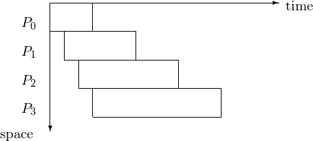
Fig. 42 Space-time diagram for pipeline with stages of varying length.
Parallel Solving
Using an n-stage pipeline, we assume that L is available on every processor.
The corresponding 4-stage pipeline is shown in Fig. 43 with the space-time diagram in Fig. 44.

Fig. 43 4-stage pipeline to solve a 4-by-4 lower triangular system.
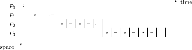
Fig. 44 Space-time diagram for solving a 4-by-4 lower triangular system.
In type 3 pipelining, a worker continues after passing results through. The making of \(y_1\) available in the next pipeline cycle is illustrated in Fig. 45. The corresponding space-time diagram is in Fig. 46 and the space-time diagram in Fig. 47 shows at what time step which component of the solution is.

Fig. 45 Passing \(y_1\) through the type 3 pipeline.
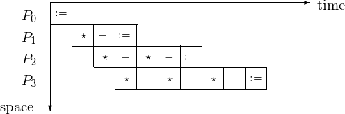
Fig. 46 Space-time diagram of a type 3 pipeline.
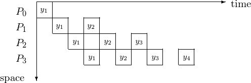
Fig. 47 Space-time diagram illustrates the component of the solutions.
We count the steps for \(p = 4\) or in general, for \(p = n\) as follows. The latency takes 4 steps for \(y_1\) to be at \(P_4\), or in general: n steps for \(y_1\) to be at \(P_n\). It takes then 6 additional steps for \(y_4\) to be computed by \(P_4\), or in general: \(2n-2\) additional steps for \(y_n\) to be computed by \(P_n\). So it takes \(n + 2n - 2 = 3n - 2\) steps to solve an n-dimensional triangular system by an n-stage pipeline.
y := b
for i from 2 to n do
    for j from i to n do
        y[j] := y[j] - L[j][i-1]*y[i-1]
Consider for example the solving of \(L {\bf y} = {\bf b}\) for \(n = 5\).
\(y := {\bf b}\);
\(y_2 := y_2 - \ell_{2,1} \star y_1\);
\(y_3 := y_3 - \ell_{3,1} \star y_1\);
\(y_4 := y_4 - \ell_{4,1} \star y_1\);
\(y_5 := y_5 - \ell_{5,1} \star y_1\);
\(y_3 := y_3 - \ell_{3,2} \star y_2\);
\(y_4 := y_4 - \ell_{4,2} \star y_2\);
\(y_5 := y_5 - \ell_{5,2} \star y_2\);
\(y_4 := y_4 - \ell_{4,3} \star y_3\);
\(y_5 := y_5 - \ell_{5,3} \star y_3\);
\(y_5 := y_5 - \ell_{5,4} \star y_4\);
Observe that all instructions in the j loop are independent from each other!
Consider the inner loop in the algorithm to solve \(L {\bf y} = {\bf b}\). We distribute the update of \(y_i, y_{i+1}, \ldots, y_n\) among p processors. If \(n \gg p\), then we expect a close to optimal speedup.
Parallel Solving with OpenMP
For our parallel solver for triangular systems, the setup is as follows. For \(L = [ \ell_{i,j} ]\), we generate random numbers for \(\ell_{i,j} \in [0,1]\). The exact solution \(\bf y\): \(y_i = 1\), for \(i=1,2,\ldots,n\). We compute the right hand side \({\bf b} = L {\bf y}\).
For dimensions \(n > 800\), hardware doubles are insufficient. With hardware doubles, the accumulation of round off is such that we loose all accuracy in \(y_n\). We recall that condition numbers of n-dimensional triangular systems can grow as large as \(2^n\). Therefore, we use quad double arithmetic.
Relying on hardware doubles is problematic:
$ time /tmp/trisol 10
last number : 1.0000000000000009e+00

real   0m0.003s    user   0m0.001s    sys   0m0.002s

$ time /tmp/trisol 100
last number : 9.9999999999974221e-01

real   0m0.005s    user   0m0.001s    sys   0m0.002s

$ time /tmp/trisol 1000
last number : 2.7244600009080568e+04

real   0m0.036s    user   0m0.025s    sys   0m0.009s
Allocating a matrix of quad double in the main program is done as follows:
{
   qd_real b[n],y[n];
   int i,j;

   qd_real **L;
   L = (qd_real**) calloc(n,sizeof(qd_real*));
   for(i=0; i<n; i++)
      L[i] = (qd_real*) calloc(n,sizeof(qd_real));

   srand(time(NULL));
   random_triangular_system(n,L,b);
The function for a random triangular system is defined next:
void random_triangular_system ( int n, qd_real **L, qd_real *b )
{
   int i,j;
   for(i=0; i<n; i++)
   {
      L[i][i] = 1.0;
      for(j=0; j<i; j++)
      {
         double r = ((double) rand())/RAND_MAX;
         L[i][j] = qd_real(r);
      }
      for(j=i+1; j<n; j++)
         L[i][j] = qd_real(0.0);
   }
   for(i=0; i<n; i++)
   {
      b[i] = qd_real(0.0);
      for(j=0; j<n; j++)
         b[i] = b[i] + L[i][j];
   }
}
Solving the system is done by the function below.
void solve_triangular_system_swapped ( int n, qd_real **L, qd_real *b, qd_real *y )
{
   int i,j;

   for(i=0; i<n; i++) y[i] = b[i];

   for(i=1; i<n; i++)
   {
      for(j=i; j<n; j++)
         y[j] = y[j] - L[j][i-1]*y[i-1];
   }
}
Now we insert the OpenMP directives:
void solve_triangular_system_swapped ( int n, qd_real **L, qd_real *b, qd_real *y )
{
   int i,j;

   for(i=0; i<n; i++) y[i] = b[i];

   for(i=1; i<n; i++)
   {
      #pragma omp parallel shared(L,y) private(j)
      {
         #pragma omp for
         for(j=i; j<n; j++)
            y[j] = y[j] - L[j][i-1]*y[i-1];
      }
   }
}
Running time /tmp/trisol_qd_omp n p,
for dimension \(n = 8,000\) for varying number p of cores
gives times as in table Table 16.
| p | cpu time | real | user | sys |
|---|---|---|---|---|
| 1 | 21.240s | 35.095s | 34.493s | 0.597s |
| 2 | 22.790s | 25.237s | 36.001s | 0.620s |
| 4 | 22.330s | 19.433s | 35.539s | 0.633s |
| 8 | 23.200s | 16.726s | 36.398s | 0.611s |
| 12 | 23.260s | 15.781s | 36.457s | 0.626s |
The serial part is the generation of the random numbers for L and the computation of \({\bf b} = L {\bf y}\). Recall Amdahl’s Law.
We can compute the serial time, subtracting for \(p=1\), from the real time the cpu time spent in the solver, i.e.: \(35.095 - 21.240 = 13.855\).
For \(p = 12\), time spent on the solver is \(15.781 - 13.855 = 1.926\). Compare 1.926 to 21.240/12 = 1.770.
Exercises
- Consider the upper triangular system \(U {\bf x} = {\bf y}\), with \(U = [u_{i,j}]\), \(u_{i,j} = 0\) if \(i > j\). Derive the formulas and general algorithm to compute the components of the solution \({\bf x}\). For \(n=4\), draw the third type of pipeline.
- Write a parallel solver with OpenMP to solve \(U {\bf x} = {\bf y}\). Take for \(U\) a matrix with random numbers in \([0,1]\), compute \({\bf y}\) so all components of \({\bf x}\) equal one. Test the speedup of your program, for large enough values of \(n\) and a varying number of cores.
- Describe a parallel solver for upper triangular systems \(U {\bf y} = {\bf b}\) for distributed memory computers. Write a prototype implementation using MPI and discuss its scalability.