Parallel Numerical Linear Algebra

QR Factorization

To solve an overconstrained linear system \(A {\bf x} = {\bf b}\) of m equations in n variables, where \(m > n\), we factor \(A\) as a product of two matrices, \(A = Q R\):

1. Q is an orthogonal matrix: \(Q^H Q = I\), the inverse of Q is its Hermitian transpose \(Q^H\);
2. R is upper triangular: \(R = [r_{i,j}]\), \(r_{i,j} = 0\) if \(i > j\).

Solving \(A {\bf x} = {\bf b}\) is equivalent to solving \(Q(R {\bf x}) = {\bf b}\). We multiply \(\bf b\) with \(Q^T\) and then apply backward substitution: \(R {\bf x} = Q^T {\bf b}\). The solution \(\bf x\) minimizes the square of the residual \(|| b - A {\bf x} ||_2^2\) (least squares).

Householder transformation

For \({\bf v} \not=0\): \(\displaystyle H = I - \frac{{\bf v} {\bf v}^T}{{\bf v}^T {\bf v}}\) is a Householder transformation.

By its definition, \(H = H^T = H^{-1}\). Because of their geometrical interpretation, Householder transformations are also called Householder reflectors.

For some n-dimensional real vector \(\bf x\), let \({\bf e}_1 = (1,0,\ldots,0)^T\):

\[{\bf v} = {\bf x} - ||{\bf x}||_2 {\bf e}_1 \quad \Rightarrow \quad H {\bf x} = ||{\bf x}||_2 {\bf e}_1.\]

With H we eliminate, reducing A to an upper triangular matrix. Householder QR: Q is a product of Householder reflectors.

The LAPACK DGEQRF on an m-by-n matrix produces:

\[H_1 H_2 \cdots H_n = I - V T V^T\]

where each \(H_i\) is a Householder reflector matrix with associated vectors \({\bf v}_i\) in the columns of V and T is an upper triangular matrix.

For an $m$-by-$n$ matrix $A = [a_{i,j}]$ with columns $bfa_j$, the formulas are formatted as pseudo code for a Householder QR factorization in Fig. 61.

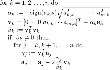
Fig. 61 Pseudo code for Househoulder QR factorization.

For a parallel implementation, we consider tiled matrices, dividing the m-by-n matrix A into b-by-b blocks, \(m = b \times p\) and \(n = b \times q\). Then we consider A as an \((p \times b)\)-by-\((q \times b)\) matrix:

\[\begin{split}A = \left[ \begin{array}{cccc} A_{1,1} & A_{1,2} & \cdots & A_{1,q} \\ A_{2,1} & A_{2,2} & \cdots & A_{2,q} \\ \vdots & \vdots & \ddots & \vdots \\ A_{p,1} & A_{p,2} & \cdots & A_{p,q} \end{array} \right],\end{split}\]

where each \(A_{i,j}\) is an b-by-b matrix. A crude classification of memory hierarchies distinguishes between registers (small), cache (medium), and main memory (large). To reduce data movements, we want to keep data in registers and cache as much as possible.

To introduce QR factorization on a tiled matrix, consider for example

\[\begin{split}A = \left[ \begin{array}{cc} A_{1,1} & A_{1,2} \\ A_{2,1} & A_{2,2} \end{array} \right] = Q \left[ \begin{array}{cc} R_{1,1} & R_{1,2} \\ 0 & R_{2,2} \end{array} \right].\end{split}\]

We proceed in three steps.

1. Perform a QR factorization:

   \[\begin{split}\begin{array}{l} A_{1,1} = Q_1 B_{1,1} \\ (Q_1,B_{1,1}) := {\rm QR}(A_{1,1}) \end{array} \quad {\rm and} \quad \begin{array}{l} A_{1,2} = Q_1 B_{1,2} \\ B_{1,2} = Q_1^T A_{1,2} \end{array}\end{split}\]

2. Coupling square blocks:

   \[\begin{split}(Q_2, R_{1,1}) := {\rm QR} \left( \left[ \begin{array}{c} B_{1,1} \\ A_{2,1} \end{array} \right] \right) \quad {\rm and} \quad \left[ \begin{array}{c} R_{1,2} \\ B_{2,2} \end{array} \right] := Q_2^T \left[ \begin{array}{c} R_{1,2} \\ A_{2,2} \end{array} \right].\end{split}\]

3. Perform another QR factorization: \((Q_3,R_{2,2}) := {\rm QR}(B_{2,2})\).

Pseudo code for a tiled QR factorization is given below.

for k from 1 to min(p,q) do
    DGEQRT(A[k][k], V[k][k], R[k][k], T[k][k])
    for i from k+1 to p do
        DLARFB(A[k][j], V[k][k], T[k][k], R[k][j])
    for i from k+1 to p do
        DTSQRT(R[k][k], A[i][k], V[i][k], T[i][k])
        for j from k+1 to p do
            DSSRFB(R[k][j], A[i][j], V[i][k], T[i][k])

where the function calls correspond to the folllowing mathematical formulas:

• DGEQRT(A[k][k], V[k][k], R[k][k], T[k][k]) corresponds to \(V_{k,k}, R_{k,k}, T_{k,k} := \mbox{QR}(A_{k,k})\).

• DLARFB(A[k]][j], V[k][k], T[k][k], R[k][j]) corresponds to \(R_{k,j} := ( I - V_{k,k} T_{k,k} V_{k,k}^T ) A_{k,j}\).

• DTSQRT(R{k][k], A[i][k], V[i][k], T[i][k]) corresponds to

  \[\begin{split}(V_{i,k},T_{i,k},R_{k,k}) := {\rm QR}\left( \left[ \begin{array}{c} \! R_{k,k} \! \\ \! A_{i,k} \! \end{array} \right] \right).\end{split}\]

• DSSRFB(R[k][j], A[i][j], V[i][k], T[i][k]) corresponds to

  \[\begin{split}\left[ \begin{array}{c} \!\! R_{k,j} \!\! \\ \!\! A_{i,j} \!\! \end{array} \right] := ( I - V_{i,k} T_{i,k} V_{i,k}^T) \left[ \begin{array}{c} \!\! R_{k,j} \!\! \\ \!\! A_{i,j} \!\! \end{array} \right].\end{split}\]

The directory examples in /usr/local/plasma-installer_2.6.0/build/plasma_2.6.0 contains example_dgeqrs, an example for solving an overdetermined linear system with a QR factorization.

Compiling on a MacBook Pro in the examples directory:

$ sudo make example_dgeqrs
gcc -O2 -DADD_ -I../include -I../quark
-I/usr/local/plasma-installer_2.6.0/install/include
-c example_dgeqrs.c -o example_dgeqrs.o
gfortran  example_dgeqrs.o -o example_dgeqrs -L../lib
-lplasma  -lcoreblasqw -lcoreblas -lplasma -L../quark
-lquark  -L/usr/local/plasma-installer_2.6.0/install/lib
-llapacke -L/usr/local/plasma-installer_2.6.0/install/lib
-ltmg  -framework veclib  -lpthread -lm
$

On kepler we do the same.

To make the program in our own home directory, we define a makefile:

PLASMA_DIR=/usr/local/plasma-installer_2.6.0/build/plasma_2.6.0

example_dgeqrs:
        gcc -O2 -DADD_ -I$(PLASMA_DIR)/include -I$(PLASMA_DIR)/quark \
            -I/usr/local/plasma-installer_2.6.0/install/include \
            -c example_dgeqrs.c -o example_dgeqrs.o
        gfortran  example_dgeqrs.o -o example_dgeqrs \
            -L$(PLASMA_DIR)/lib -lplasma -lcoreblasqw \
            -lcoreblas -lplasma -L$(PLASMA_DIR)/quark -lquark \
            -L/usr/local/plasma-installer_2.6.0/install/lib -lcblas \
            -L/usr/local/plasma-installer_2.6.0/install/lib -llapacke \
            -L/usr/local/plasma-installer_2.6.0/install/lib -ltmg -llapack \
            -L/usr/local/plasma-installer_2.6.0/install/lib \
            -lrefblas -lpthread -lm

Typing make example_dgeqrs will then compile and link. Running example_dgeqrs with dimension 4000:

$ time ./example_dgeqrs
-- PLASMA is initialized to run on 1 cores.
============
Checking the Residual of the solution
-- ||Ax-B||_oo/((||A||_oo||x||_oo+||B||)_oo.N.eps) = 2.829153e-02
-- The solution is CORRECT !
-- Run of DGEQRS example successful !

real    0m42.172s
user    0m41.965s
sys     0m0.111s
$

Results of time example_dgeqrs, for dimension 4000, are listed in Table 21.

Table 21 Timings on dgeqrs for n = 4000, with p threads.

p	real	user	sys	speedup
1	42.172	41.965	0.111
2	21.495	41.965	0.154	1.96
4	11.615	43.322	0.662	3.63
8	6.663	46.259	1.244	6.33
16	3.872	46.793	2.389	10.89

Conjugate Gradient and Krylov Subspace Methods

We link linear systems solving to an optimization problem. Let A be a positive definite matrix: \(\forall {\bf x}: {\bf x}^T A {\bf x} \geq 0\) and \(A^T = A\). The optimum of

\[q({\bf x}) = \frac{1}{2} {\bf x}^T A {\bf x} - {\bf x}^T {\bf b} \mbox{ is at } A {\bf x} - {\bf b} = {\bf 0}.\]

For the exact solution \(\bf x\): \(A {\bf x} = {\bf b}\) and an approximation \({\bf x}_k\), let the error be \({\bf e}_k = {\bf x}_k - {\bf x}\).

\[\begin{split}\begin{array}{lcr} || {\bf e}_k ||_A^2 ~~= ~~ {\bf e}_k^T A {\bf e}_k & = & ({\bf x}_k - {\bf x})^T A ({\bf x}_k - {\bf x}) \\ & = & {\bf x}_k^T A {\bf x}_k - 2 {\bf x}_k^T A {\bf x} + {\bf x}^T A {\bf x} \\ & = & {\bf x}_k^T A {\bf x}_k - 2 {\bf x}_k^T {\bf b} + c \\ & = & 2 q({\bf x}_k) + c \end{array}\end{split}\]

\(\Rightarrow\) minimizing \(q({\bf x})\) is the same as minimizing the error.

The conjugate gradient method is similar to the steepest descent method, formulated in Fig. 62.

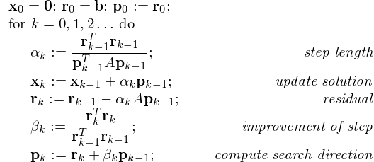
Fig. 62 Mathematical definition of the conjugate gradient method.

For large sparse matrices, the conjugate gradient method is much faster than Cholesky.

Krylov subspace methods

We consider spaces spanned by matrix-vector products.

• Input: right hand side vector \(\bf b\) of dimension n, and some algorithm to evaluate \(A {\bf x}\).
• Output: approximation for \(A^{-1} {\bf b}\).

Example (\(n=4\)), consider \({\bf y}_1 = {\bf b}\), \({\bf y}_2 = A {\bf y}_1\), \({\bf y}_3 = A {\bf y}_2\), \({\bf y}_4 = A {\bf y}_3\), stored in the columns of \(K = [{\bf y}_1 ~ {\bf y}_2 ~ {\bf y}_3 ~ {\bf y}_4]\).

\[\begin{split}\begin{array}{lcr} A K & = & [A {\bf y}_1 ~ A {\bf y}_2 ~ A {\bf y}_3 ~ A {\bf y}_4] ~~ = ~~ [{\bf y}_2 ~ {\bf y}_3 ~ {\bf y}_4 ~ A^4 {\bf y}_1 ] \\ & = & K \left[ \begin{array}{cccc} 0 & 0 & 0 & -c_1 \\ 1 & 0 & 0 & -c_2 \\ 0 & 1 & 0 & -c_3 \\ 0 & 0 & 1 & -c_4 \\ \end{array} \right], \quad {\bf c} = - K^{-1} A^4 {\bf y}_1. \end{array}\end{split}\]

\(\Rightarrow AK = KC\), where \(C\) is a companion matrix.

Set \(K = [ {\bf b} ~~ A {\bf b} ~~ A^2 {\bf b} ~~ \cdots ~~ A^k {\bf b}]\). Compute \(K = QR\), then the columns of Q span the Krylov subspace. Look for an approximate solution of \(A {\bf x} = {\bf b}\) in the span of the columns of Q. We can interpret this as a modified Gram-Schmidt method, stopped after k projections of \(\bf b\).

The conjugate gradient and Krylov subspace methods rely mostly on matrix-vector products. Parallel implementations involve the distribution of the matrix among the processors. For general matrices, tiling scales best. For specific sparse matrices, the patterns of the nonzero elements will determine the optimal distribution.

PETSc (see Lecture 20) provides a directory of examples ksp of Krylov subspace methods. We will take ex3 of /usr/local/petsc-3.4.3/src/ksp/ksp/examples/tests To get the makefile, we compile in the examples and then copy the compilation and linking instructions. The makefile on kepler looks as follows:

PETSC_DIR=/usr/local/petsc-3.4.3
PETSC_ARCH=arch-linux2-c-debug

ex3:
        $(PETSC_DIR)/$(PETSC_ARCH)/bin/mpicc -o ex3.o -c -fPIC -Wall \
        -Wwrite-strings -Wno-strict-aliasing -Wno-unknown-pragmas -g3 \
        -fno-inline -O0   -I/usr/local/petsc-3.4.3/include \
        -I/usr/local/petsc-3.4.3/arch-linux2-c-debug/include \
        -D__INSDIR__=src/ksp/ksp/examples/tests/ ex3.c
        $(PETSC_DIR)/$(PETSC_ARCH)/bin/mpicc -fPIC -Wall -Wwrite-strings \
        -Wno-strict-aliasing -Wno-unknown-pragmas -g3 -fno-inline -O0 \
        -o ex3 ex3.o \
        -Wl,-rpath,/usr/local/petsc-3.4.3/arch-linux2-c-debug/lib \
        -L/usr/local/petsc-3.4.3/arch-linux2-c-debug/lib  -lpetsc \
        -Wl,-rpath,/usr/local/petsc-3.4.3/arch-linux2-c-debug/lib \
        -lflapack -lfblas -lX11 -lpthread -lm \
        -Wl,-rpath,/usr/gnat/lib/gcc/x86_64-pc-linux-gnu/4.7.4 \
        -L/usr/gnat/lib/gcc/x86_64-pc-linux-gnu/4.7.4 \
        -Wl,-rpath,/usr/gnat/lib64 -L/usr/gnat/lib64 \
        -Wl,-rpath,/usr/gnat/lib -L/usr/gnat/lib -lmpichf90 -lgfortran \
        -lm -Wl,-rpath,/usr/lib/gcc/x86_64-redhat-linux/4.4.7 \
        -L/usr/lib/gcc/x86_64-redhat-linux/4.4.7 -lm -lmpichcxx -lstdc++ \
        -ldl -lmpich -lopa -lmpl -lrt -lpthread -lgcc_s -ldl
        /bin/rm -f ex3.o

Running the example produces the following:

# time /usr/local/petsc-3.4.3/arch-linux2-c-debug/bin/mpiexec \
-n 16 ./ex3 -m 200
Norm of error 0.000622192 Iterations 162
real    0m1.855s    user    0m9.326s      sys    0m4.352s
# time /usr/local/petsc-3.4.3/arch-linux2-c-debug/bin/mpiexec \
-n 8 ./ex3 -m 200
Norm of error 0.000387934 Iterations 131
real    0m2.156s    user    0m10.363s     sys    0m1.644s
# time /usr/local/petsc-3.4.3/arch-linux2-c-debug/bin/mpiexec \
-n 4 ./ex3 -m 200
Norm of error 0.00030938 Iterations 105
real    0m4.526s    user    0m15.108s     sys     0m1.123s
# time /usr/local/petsc-3.4.3/arch-linux2-c-debug/bin/mpiexec \
-n 2 ./ex3 -m 200
Norm of error 0.000395339 Iterations 82
real    0m20.606s   user    0m37.036s     sys     0m1.996s
# time /usr/local/petsc-3.4.3/arch-linux2-c-debug/bin/mpiexec \
-n 1 ./ex3 -m 200
Norm of error 0.000338657 Iterations 83
real    1m34.991s   user    1m25.251s     sys     0m9.579s

Bibliography

1. S. Balay, J. Brown, K. Buschelman, V. Eijkhout, W. Gropp, D. Kaushik, M. Knepley, L. Curfman McInnes, B. Smith, and H. Zhang. PETSc Users Manual. Revision 3.4. Mathematics and Computer Science Division, Argonne National Laboratory, 15 October 2013.
2. E. Agullo, J. Dongarra, B. Hadri, J. Kurzak, J. Langou, H. Ltaief, P. Luszczek, and A. YarKhan. PLASMA Users’ Guide. Parallel Linear Algebra Software for Multicore Architectures. Version 2.0.
3. A. Buttari, J. Langou, J. Kurzak, and J. Dongarra. A class of parallel tiled linear algebra algorithms for multicore architectures. Parallel Computing 35: 38-53, 2009.

Exercises

1. Take a 3-by-3 block matrix, apply the tiled QR algorithm step by step, indicating which block is processed in each step along with the type of operations. Draw a Directed Acyclic Graph linking steps that have to wait on each other. On a 3-by-3 block matrix, what is the number of cores needed to achieve the best speedup?
2. Using the time command to measure the speedup of example_dgeqrs also takes into account all operations to define the problem and to test the quality of the solution. Run experiments with modifications of the source code to obtain more accurate timings of the parallel QR factorization.