Parallel Gaussian Elimination
LU and Cholesky Factorization
Consider as given a square n-by-n matrix A and corresponding right hand side vector \(\bf b\) of length n. To solve an n-dimensional linear system \(A {\bf x} = {\bf b}\) we factor A as a product of two triangular matrices, \(A = L U\):
- L is lower triangular, \(L = [\ell_{i,j}]\), \(\ell_{i,j} = 0\) if \(j > i\) and \(\ell_{i,i} = 1\).
- U is upper triangular \(U = [u_{i,j}]\), \(u_{i,j} = 0\) if \(i > j\).
Solving \(A {\bf x} = {\bf b}\) is then equivalent to solving \(L(U {\bf x}) = {\bf b}\) in two stages:
- Forward substitution: \(L {\bf y} = {\bf b}\).
- Backward substitution: \(U {\bf x} = {\bf y}\).
Factoring A costs \(O(n^3)\), solving triangular systems costs \(O(n^2)\). For numerical stability, we apply partial pivoting and compute \(PA = LU\), where P is a permutation matrix.
The steps in the LU factorization of the matrix A are shown in Fig. 59.
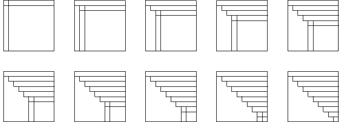
Fig. 59 Steps in the LU factorization.
For column \(j = 1,2,\ldots,n-1\) in A do
- find the largest element \(a_{i,j}\) in column \(j\) (for \(i \geq j\));
- if \(i \not= j\), then swap rows \(i\) and \(j\);
- for \(i = j+1, \ldots n\), for \(k=j+1,\ldots,n\) do \(\displaystyle a_{i,k} := a_{i,k} - \left( \frac{a_{i,j}}{a_{j,j}} \right) a_{j,k}\).
If \(A\) is symmetric, \(A^T = A\), and positive semidefinite: \(\forall {\bf x}: {\bf x}^T A {\bf x} \geq 0\), then we better compute a Cholesky factorization: \(A = L L^T\), where \(L\) is a lower triangular matrix. Because \(A\) is positive semidefinite, no pivoting is needed, and we need about half as many operations as LU.
Pseudo code is listed below:
for j from 1 to n do
    for k from 1 to j-1 do
        a[j][j] := a[j][j] - a[j][k]**2
    a[j][j] := sqrt(a[j][j])
    for i from j+1 to n do
        for k from 1 to j do
            a[i][j] := a[i][j] - a[i][k]*a[j][k]
        a[i][j] := a[i][j]/a[j][j]
Let A be a symmetric, positive definite n-by-n matrix. In preparation for parallel implementation, we consider tiled matrices. For tile size b, let \(n = p \times b\) and consider
where \(A_{i,j}\) is an b-by-b matrix.
A crude classification of memory hierarchies distinguishes between registers (small), cache (medium), and main memory (large). To reduce data movements, we want to keep data in registers and cache as much as possible.
Pseudo code for a tiled Cholesky factorization is listed below.
for k from 1 to p do
    DPOTF2(A[k][k], L[k][k])                 # L[k][k] := Cholesky(A[k][k])
    for i from k+1 to p do
        DTRSM(L[k][k], A[i][k], L[i][k])     # L[i][k] := A[i][k]*L[k][k]**(-T)
    end for
    for i from k+1 to p do
        for j from k+1 to p do
            DGSMM(L[i][k], L[j][k], A[i][j]) # A[i][j] := A[i][j] - L[i][k]*L[j][k]}**T
        end for
end for
Blocked LU Factorization
In deriving blocked formulations of LU, consider a 3-by-3 blocked matrix. The optimal size of the blocks is machine dependent.
Expanding the right hand side and equating to the matrix at the left gives formulations for the LU factorization.
The formulas we are deriving gives rise to the right looking LU. We store the \(L_{i,j}\)‘s and \(U_{i,j}\)‘s in the original matrix:
The matrices \(B_{i,j}\)‘s are obtained after a first block LU step. To find \(L_{2,2}\), \(L_{3,2}\), and \(U_{2,2}\) we use
- Eliminating \(A_{2,2} - L_{2,1} U_{1,2}\)
- and \(A_{3,2} - L_{3,1} U_{1,2}\) gives
Via LU on \(B_{2,2}\) we obtain \(L_{2,2}\) and \(U_{2,2}\). Then: \(L_{3,2} := B_{3,2} U_{2,2}^{-1}\).
The formulas we derived are similar to the scalar case and are called right looking.
But we may organize the LU factorization differently, as shown in Fig. 60.
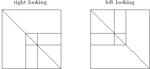
Fig. 60 Right and left looking organization of tiled LU factorization.
What is good looking? Left is best for data access. We derive left looking formulas. Going from \(P_1 A\) to \(P_2 P_1 A\):
We keep the original \(A_{i,j}\)‘s and postpone updating to the right.
We get \(U_{1,2}\) via \(A_{1,2} = L_{1,1} U_{1,2}\) and compute \(U_{1,2} = L_{1,1}^{-1} A_{1,2}\).
To compute \(L_{2,2}\) and \(L_{3,2}\) do \(\displaystyle \left[ \begin{array}{c} B_{2,2} \\ B_{3,2} \end{array} \right] = \left[ \begin{array}{c} A_{2,2} \\ A_{3,2} \end{array} \right] - \left[ \begin{array}{c} L_{2,1} \\ L_{3,1} \end{array} \right] U_{1,2}\);
and factor \(\displaystyle P_2 \left[ \begin{array}{c} B_{2,2} \\ B_{3,2} \end{array} \right] = \left[ \begin{array}{c} L_{2,2} \\ L_{3,2} \end{array} \right] U_{2,2}\) as before.
Replace \(\displaystyle \left[ \begin{array}{c} A_{2,3} \\ A_{3,3} \end{array} \right] := P_2 \left[ \begin{array}{c} A_{2,3} \\ A_{3,3} \end{array} \right]\) and \(\displaystyle \left[ \begin{array}{c} L_{2,1} \\ L_{3,1} \end{array} \right] := P_2 \left[ \begin{array}{c} L_{2,1} \\ L_{3,1} \end{array} \right]\).
Pseudo code for the tiled algorithm for LU factorization is below.
for k from 1 to p do
    DGETF(A[k][k], L[k][k], U[k][k], P[k][k])
    for j from k+1 to p do
        DGESSM(A[k][j], L[k][k], P[k][k], U[k][j])
    for i from k+1 to p do
        DTSTRF(U[k][k], A[i][k], P[i][k])
        for j from k+1 to p do
            DSSSM(U[k][j], A[i][j], L[i][k], P[i][k])
where the function calls correspond to the following formulas:
DGETF(A[k][k], L[k][k], U[k][k], P[k][k])corresponds to \(L_{k,k}, U_{k,k}, P_{k,k} := \mbox{LU}(A_{k,k})\).DGESSM(A[k][j], L[k][k], P[k][k], U[k][j])corresponds to \(U_{k,j} := L_{k,k}^{-1} P_{k,k} A_{k,j}\).DTSTRF(U[k][k], A[i][k], P[i][k])corresponds to \(\displaystyle U_{k,k}, L_{i,k}, P_{i,k} := LU \left( \left[ \begin{array}{c} U_{k,k} \\ A_{i,k} \end{array} \right] \right)\)DSSSM(U[k][j], A[i][j], L[i][k], P[i][k])corresponds to \(\displaystyle \left[ \begin{array}{c} U_{k,j} \\ A_{i,j} \end{array} \right] := L_{i,k}^{-1} P_{i,k} \left[ \begin{array}{c} U_{k,j} \\ A_{i,j} \end{array} \right]\).
The PLASMA Software Library
PLASMA stands for Parallel Linear Algebra Software for Multicore Architectures. The software uses FORTRAN and C. It is designed for efficiency on homogeneous multicore processors and multi-socket systems of multicore processors, Built using a small set of sequential routines as building blocks, referred to as core BLAS, and free to download from <http://icl.cs.utk.edu/plasma>.
Capabilities and limitations: Can solve dense linear systems and least squares problems. Unlike LAPACK, PLASMA currently does not solve eigenvalue or singular value problems and provide no support for band matrices.
Basic Linear Algebra Subprograms: BLAS
- Level-1 BLAS: vector-vector operations, \(O(n)\) cost. inner products, norms, \({\bf x} \pm {\bf y}\), \(\alpha {\bf x} + {\bf y}\).
- Level-2 BLAS: matrix-vector operations, \(O(mn)\) cost.
- \({\bf y} = \alpha A {\bf x} + \beta {\bf y}\)
- \(A = A + \alpha {\bf x} {\bf y}^T\), rank one update
- :math:{bf x} = T^{-1} {bf b}`, for \(T\) a triangular matrix
- Level-3 BLAS: matrix-matrix operations, \(O(kmn)\) cost.
- \(C = \alpha AB + \beta C\)
- \(C = \alpha AA^T + \beta C\), rank k update of symmetric matrix
- \(B = \alpha T B\), for \(T\) a triangular matrix
- \(B = \alpha T^{-1} B\), solve linear system with many right hand sides
The execution is asynchronous and graph driven. We view a blocked algorithm as a Directed Acyclic Graph (DAG): nodes are computational tasks performed in kernel subroutines; edges represent the dependencies among the tasks. Given a DAG, tasks are scheduled asynchronously and independently, considering the dependencies imposed by the edges in the DAG. A critical path in the DAG connects those nodes that have the highest number of outgoing edges. The scheduling policy assigns higher priority to those tasks that lie on the critical path.
The directory examples in
/usr/local/plasma-installer_2.6.0/build/plasma_2.6.0
contains
example_cposv, an example for a Cholesky factorization
of a symmetric positive definite matrix.
Running make as defined in the examples directory:
[root@kepler examples]# make example_cposv
gcc -O2 -DADD_ -I../include -I../quark \
-I/usr/local/plasma-installer_2.6.0/install/include -c \
example_cposv.c -o example_cposv.o
gfortran  example_cposv.o -o example_cposv -L../lib -lplasma \
-lcoreblasqw -lcoreblas -lplasma -L../quark -lquark \
-L/usr/local/plasma-installer_2.6.0/install/lib -lcblas \
-L/usr/local/plasma-installer_2.6.0/install/lib -llapacke \
-L/usr/local/plasma-installer_2.6.0/install/lib -ltmg -llapack \
-L/usr/local/plasma-installer_2.6.0/install/lib -lrefblas \
-lpthread -lm
[root@kepler examples]#
Cholesky factorization with the dimension equal to 10,000.
[root@kepler examples]# time ./example_dposv
-- PLASMA is initialized to run on 2 cores.
============
Checking the Residual of the solution
-- ||Ax-B||_oo/((||A||_oo||x||_oo+||B||_oo).N.eps) = 2.710205e-03
-- The solution is CORRECT !
-- Run of DPOSV example successful !

real    1m22.271s
user    2m42.534s
sys     0m1.064s
[root@kepler examples]#
The wall clock times for Cholesky on dimension 10,000 are listed in Table 20.
| #cores | real time | speedup |
|---|---|---|
| 1 | 2m 40.913s | |
| 2 | 1m 22.271s | 1.96 |
| 4 | 42.621s | 3.78 |
| 8 | 23.480s | 6.85 |
| 16 | 12.647s | 12.72 |
Bibliography
- E. Agullo, J. Dongarra, B. Hadri, J. Kurzak, J. Langou, H. Ltaief, P. Luszczek, and A. YarKhan. PLASMA Users’ Guide. Parallel Linear Algebra Software for Multicore Architectures. Version 2.0.
- A. Buttari, J. Langou, J. Kurzak, and J. Dongarra. A class of parallel tiled linear algebra algorithms for multicore architectures. Parallel Computing 35: 38-53, 2009.
Exercises
- Write your own parallel shared memory version of the Cholesky factorization, using OpenMP, Pthreads, or the Intel TBB.
- Derive right looking LU factorization formulas with pivoting, i.e.: introducing permutation matrices P. Develop first the formulas for a 3-by-3 block matrix and then generalize the formulas into an algorithm for any p-by-p block matrix.
- Take an appropriate example from the PLASMA installation to test the speedup of the multicore LU factorization routines.