Domain Decomposition Methods

THe method of Jacobi is an interative method which is not in place: we do not overwrite the current solution with new components as soon as these become available. In contrast, the method of Gauss-Seidel does update the current solution with newly computed components of the solution as soon as these are computed.

Domain decomposition methods to solve partial differential equations are another important class of synchronized parallel computations, explaining the origin for the need to solve large linear systems. This chapter ends with an introduction to the software PETSc, the Portable, Extensible Toolkit for Scientific Computation.

Gauss-Seidel Relaxation

The method of Gauss-Seidel is an iterative method for solving linear systems. We want to solve \(A {\bf x} = {\bf b}\) for a very large dimension n. Writing the method of Jacobi componentwise:

\[x_i^{(k+1)} := x_i^{(k)} + \frac{1}{a_{i,i}} \left( b_i - \sum_{j=1}^n a_{i,j} x_j^{(k)} \right), \quad i=1,2,\ldots,n\]

We observe that we can already use \(x_j^{(k+1)}\) for \(j < i\). This leads to the following formulas

\[x_i^{(k+1)} := x_i^{(k)} + \frac{1}{a_{i,i}} \left( b_i - \sum_{j=1}^{i-1} a_{i,j} x_j^{(k+1)} - \sum_{j=i}^n a_{i,j} x_j^{(k)} \right), \quad i=1,2,\ldots,n.\]

C code for the Gauss-Seidel method is below.

void run_gauss_seidel_method
 ( int n, double **A, double *b, double epsilon, int maxit, int *numit, double *x )
/*
 * Runs the  method of Gauss-Seidel for A*x = b.
 *
 * ON ENTRY :
 *   n        the dimension of the system;
 *   A        an n-by-n matrix A[i][i] /= 0;
 *   b        an n-dimensional vector;
 *   epsilon  accuracy requirement;
 *   maxit    maximal number of iterations;
 *   x        start vector for the iteration.
 *
 * ON RETURN :
 *   numit    number of iterations used;
 *   x        approximate solution to A*x = b. */
{
   double *dx = (double*) calloc(n,sizeof(double));
   int i,j,k;
   for(k=0; k<maxit; k++)
   {
      double sum = 0.0;
      for(i=0; i<n; i++)
      {
         dx[i] = b[i];
         for(j=0; j<n; j++)
            dx[i] -= A[i][j]*x[j];
         dx[i] /= A[i][i]; x[i] += dx[i];
         sum += ( (dx[i] >= 0.0) ? dx[i] : -dx[i]);
      }
      printf("%4d : %.3e\n",k,sum);
      if(sum <= epsilon) break;
   }
   *numit = k+1; free(dx);
}

Running on the same example as in the previous chapter goes much faster:

$ time /tmp/gauss_seidel 1000
   0 : 1.264e+03
   1 : 3.831e+02
   2 : 6.379e+01
   3 : 1.394e+01
   4 : 3.109e+00
   5 : 5.800e-01
   6 : 1.524e-01
   7 : 2.521e-02
   8 : 7.344e-03
   9 : 1.146e-03
  10 : 3.465e-04
  11 : 5.419e-05
computed 12 iterations     <----- 8407 with Jacobi
error : 1.477e-05

real    0m0.069s           <----- 0m42.411s
user    0m0.063s           <----- 0m42.377s
sys     0m0.005s           <----- 0m0.028s

Parallel Gauss-Seidel with OpenMP

Using p threads:

void run_gauss_seidel_method
 ( int p, int n, double **A, double *b, double epsilon, int maxit, int *numit, double *x )
{
   double *dx;
   dx = (double*) calloc(n,sizeof(double));
   int i,j,k,id,jstart,jstop;

   int dnp = n/p;
   double dxi;

   for(k=0; k<maxit; k++)
   {
      double sum = 0.0;
      for(i=0; i<n; i++)
      {
         dx[i] = b[i];
         #pragma omp parallel shared(A,x) private(id,j,jstart,jstop,dxi)
         {
            id = omp_get_thread_num();
            jstart = id*dnp;
            jstop = jstart + dnp;
            dxi = 0.0;
            for(j=jstart; j<jstop; j++)
               dxi += A[i][j]*x[j];
            #pragma omp critical
               dx[i] -= dxi;
         }
      }
   }
}

Observe that although the entire matrix A is shared between all threads, each threads needs only n/p columns of the matrix. In the MPI version of the method of Jacobi, entire rows of the matrix were distributed among the processors. If we were to make a distributed memory version of the OpenMP code, then we would distribute entire columns of the matrix A over the processors.

Running times obtained via the command time are in Table 19.

Table 19 Times of a parallel Gauss-Seidel with OpenMP

p	n	real	user	sys	speedup
1	10,000	7.165s	6.921s	0.242s
	20,000	28.978s	27.914s	1.060s
	30,000	1m 6.491s	1m 4.139s	2.341s
2	10,000	4.243s	7.621s	0.310s	1.689
	20,000	16.325s	29.556s	1.066s	1.775
	30,000	36.847s	1m 6.831s	2.324s	1.805
5	10,000	2.415s	9.440s	0.420s	2.967
	20,000	8.403s	32.730s	1.218s	3.449
	30,000	18.240s	1m 11.031s	2.327s	3.645
10	10,000	2.173s	16.241s	0.501s	3.297
	20,000	6.524s	45.629s	1.521s	4.442
	30,000	13.273s	1m 29.687s	2.849s	5.010

Solving the Heat Equation

We will be applying a time stepping method to the heat or diffusion equation:

\[\frac{\partial^2 u}{\partial x^2} + \frac{\partial^2 u}{\partial y^2} = \frac{\partial u}{\partial t}\]

models the temperature distribution \(u(x,y,t)\) evolving in time \(t\) for \((x,y)\) in some domain.

Related Partial Differential Equations (PDEs) are

\[\frac{\partial^2 u}{\partial x^2} + \frac{\partial^2 u}{\partial y^2} = 0 \quad {\rm and} \quad \frac{\partial^2 u}{\partial x^2} + \frac{\partial^2 u}{\partial y^2} = f(x,y),\]

respectively called the Laplace and Poisson equations.

For the discretization of the derivatives, consider that at a point \((x_0,y_0,t_0)\), we have

\[\left. \frac{\partial u}{\partial x} \right|_{(x_0,y_0,t_0)} = \lim_{h \rightarrow 0} ~ \underbrace{\frac{u(x_0+h,y_0,t_0) - u(x_0,y_0,h)}{h}}_{u_x(x_0,y_0,t_0)}\]

so for positive \(h \approx 0\), \(\displaystyle u_x(x_0,y_0,t_0) \approx \left. \frac{\partial u}{\partial x} \right|_{(x_0,y_0,t_0)}\).

For the second derivative we use the finite difference \(u_{xx}(x_0,y_0,t_0)\)

\[\begin{split}\begin{array}{rcl} \!\!\! & = & {\displaystyle \frac{1}{h} \left( \frac{u(x_0 + h,y_0,t_0) - u(x_0,y_0,t_0)}{h} - \frac{u(x_0,y_0,t_0) - u(x_0-h,y_0,t_0)}{h} \right)} \\ \!\!\! & = & {\displaystyle \frac{u(x_0 + h,y_0,t_0) - 2 u(x_0,y_0,t_0) + u(x_0-h,y_0,t_0)}{h^2}}. \end{array}\end{split}\]

Time stepping is then done along the formulas:`

\[\begin{split}\begin{array}{rcl} u_t(x_0,y_0,t_0) & = & {\displaystyle \frac{u(x_0,y_0,t_0+h) - u(x_0,y_0,t_0)}{h}} \\ u_{xx}(x_0,y_0,t_0) & = & {\displaystyle \frac{u(x_0+h,y_0,t_0) - 2 u(x_0,y_0,t_0) + u(x_0-h,y_0,t_0)}{h^2}} \\ u_{yy}(x_0,y_0,t_0) & = & {\displaystyle \frac{u(x_0,y_0+h,t_0) - 2 u(x_0,y_0,t_0) + u(x_0,y_0-h,t_0)}{h^2}} \end{array}\end{split}\]

Then the equation \(\displaystyle \frac{\partial u}{\partial t} = \frac{\partial^2 u}{\partial x^2} + \frac{\partial^2 u}{\partial y^2}\) becomes

\[\begin{split}\begin{array}{rcl} u(x_0,y_0,t_0+h) & \!\! = \!\! & u(x_0,y_0,t_0) \\ & \!\! + \!\! & {\displaystyle h ~ \left[ ~ u(x_0+h,y_0,t_0) + u(x_0-h,y_0,t_0) \right.} \\ & \!\! + \!\! & ~~~~ {\displaystyle \left. u(x_0,y_0+h,t_0) + u(x_0,y_0-h,t_0) - 4 u(x_0,y_0,t_0) ~ \right]} \end{array}\end{split}\]

Locally, the error of this approximation is \(O(h^2)\).

The algorithm performs synchronous iterations on a grid. For \((x,y) \in [0,1] \times [0,1]\), the division of \([0,1]\) in n equal subintervals, with \(h = 1/n\), leads to a grid \((x_i = ih, y_j = jh)\), for \(i=0,1,\ldots,n\) and \(j=0,1,\ldots,n\). For t, we use the same step size h: \(t_k = kh\). Denote \(u_{i,j}^{(k)} = u(x_i,y_j,t_k)\), then

\[u_{i,j}^{(k+1)} = u_{i,j}^{(k)} + h ~ \left[ ~ u_{i+1,j}^{(k)} + u_{i-1,j}^{(k)} + u_{i,j+1}^{(k)} + u_{i,j-1}^{(k)} - 4 u_{i,j}^{(k)} ~ \right].\]

Fig. 56 shows the labeling of the grid points.

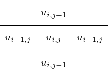
Fig. 56 In every step, we update \(u_{i,j}\) based on \(u_{i-1,j}\), \(u_{i+1,j}\), \(u_{i,j-1}\), and \(u_{i,j+1}\).

We divide the grid in red and black points, as in Fig. 57.

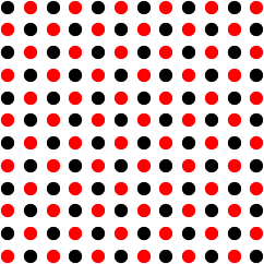
Fig. 57 Organization of the grid \(u_{i,j}\) in red and black points.

The computation is organized in two phases:

1. In the first phase, update all black points simultaneously; and then
2. in the second phase, update all red points simultaneously.

domain decomposition

We can decompose a domain in strips, but then there are $n/p$ boundaries that must be shared. To reduce the overlapping, we partition in squares, as shown in Fig. 58.

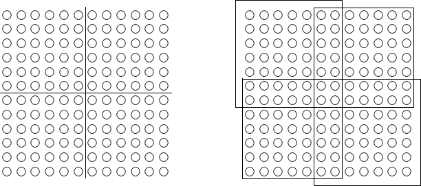
Fig. 58 Partitioning of the grid in squares.

Then the boundary elements are proportional to \(n/\sqrt{p}\).

In Fig. 58, two rows and two columns are shared between two partitions. To reduce the number of shared rows and columns to one, we can take an odd number of rows and columns. In the example of Fig. 58, instead of 12 rows and columns, we could take 11 or 13 rows and columns. Then only the middle row and column is shared between the partitions.

Comparing communication costs, we make the following observations. In a square partition, every square has 4 edges, whereas a strip has only 2 edges. For the communication cost, we multiply by 2 because for every send there is a receive. Comparing the communication cost for a strip partitioning

\[t_{\rm comm}^{\rm strip} = 4 \left( t_{\rm startup} + n t_{\rm data} \right)\]

to the communication cost for a square partitioning (for \(p \geq 9\)):

\[t_{\rm comm}^{\rm square} = 8 \left( t_{\rm startup} + \frac{n}{\sqrt{p}} t_{\rm data} \right).\]

A strip partition is best if the startup time is large and if we have only very few processors.

If the startup time is low, and for \(p \geq 4\), a square partition starts to look better.

Solving the Heat Equation with PETSc

The acronym PETSc stands for Portable, Extensible Toolkit for Scientific Computation. PETSc provides data structures and routines for large-scale application codes on parallel (and serial) computers, using MPI. It supports Fortran, C, C++, Python, and MATLAB (serial) and is free and open source, available at <http://www.mcs.anl.gov/petsc/>.

PETSc is installed on kepler in the directory /home/jan/Downloads/petsc-3.7.4. The source code contains the directory ts on time stepping methods. We will run ex3 from /home/jan/Downloads/petsc-3.7.4/src/ts/examples/tutorials After making the code, a sequential run goes like

$ /tmp/ex3 -draw_pause 1

The entry in a makefile to compile ex3:

PETSC_DIR=/usr/local/petsc-3.7.4
PETSC_ARCH=arch-linux2-c-debug

ex3:
        $(PETSC_DIR)/$(PETSC_ARCH)/bin/mpicc ex3.c \
        -I$(PETSC_DIR)/include \
        $(PETSC_DIR)/$(PETSC_ARCH)/lib/libpetsc.so \
        $(PETSC_DIR)/$(PETSC_ARCH)/lib/libopa.so \
        $(PETSC_DIR)/$(PETSC_ARCH)/lib/libfblas.a \
        $(PETSC_DIR)/$(PETSC_ARCH)/lib/libflapack.a \
        /usr/lib64/libblas.so.3 \
        -L/usr/X11R6/lib -lX11 -lgfortran -o /tmp/ex3

On a Mac OS X laptop, the PETSC_ARCH will be PETSC_ARCH=arch-darwin-c-debug.

Bibliography

1. S. Balay, J. Brown, K. Buschelman, V. Eijkhout, W. Gropp, D.~Kaushik, M. Knepley, L. Curfman McInnes, B. Smith, and H.~Zhang. PETSc Users Manual. Revision 3.2. Mathematics and Computer Science Division, Argonne National Laboratory, September 2011.
2. Ronald F. Boisvert, L. A. Drummond, Osni A. Marques: Introduction to the special issue on the Advanced CompuTational Software (ACTS) collection. ACM TOMS 31(3):281–281, 2005. Special issue on the Advanced CompuTational Software (ACTS) Collection.

Exercises

1. Take the running times of the OpenMP version of the method of Gauss-Seidel and compute the efficiency for each of the 9 cases. What can you conclude about the scalability?
2. Use MPI to write a parallel version of the method of Gauss-Seidel. Compare the speedups with the OpenMP version.
3. Run an example of the PETSc tutorials collection with an increasing number of processes to investigate the speedup.