Parallel Iterative Methods for Linear Systems

We consider the method of Jacobi and introduce the MPI_Allgather command for the synchronization of the iterations. In the analysis of the communication and the computation cost, we determine the optimal value for the number of processors which minimizes the total cost.

Jacobi Iterations

We derive the formulas for Jacobi’s method, starting from a fixed point formula. We want to solve \(A {\bf x} = {\bf b}\) for A an n-by-n matrix, and \(\bf b\) an n-dimensional vector, for very large n. Consider \(A = L + D + U\), where

• \(L = [\ell_{i,j}], \ell_{i,j} = a_{i,j}, i > j\), \(\ell_{i,j} = 0, i \leq j\). L is lower triangular.
• \(D = [d_{i,j}], d_{i,i} = a_{i,i} \not=0, d_{i,j} = 0, i \not= j\). D is diagonal.
• \(U = [u_{i,j}], u_{i,j} = a_{i,j}, i < j, u_{i,j} = 0, i \geq j\). U is upper triangular.

Then we rewrite \(A {\bf x} = {\bf b}\) as

\[\begin{split}\begin{array}{rcl} A {\bf x} = {\bf b} & \Leftrightarrow & (L + D + U) {\bf x} = {\bf b} \\ & \Leftrightarrow & D {\bf x} = {\bf b} - L {\bf x} - U {\bf x} \\ & \Leftrightarrow & D {\bf x} = D {\bf x} + {\bf b} - L {\bf x} - U {\bf x} - D {\bf x} \\ & \Leftrightarrow & D {\bf x} = D {\bf x} + {\bf b} - A {\bf x} \\ & \Leftrightarrow & {\bf x} = {\bf x} + D^{-1} ( {\bf b} - A {\bf x} ). \end{array}\end{split}\]

The fixed point formula \({\bf x} = {\bf x} + D^{-1} ( {\bf b} - A {\bf x} )\) is well defined if \(a_{i,i} \not= 0\). The fixed point formula \({\bf x} = {\bf x} + D^{-1} ( {\bf b} - A {\bf x} )\) leads to

\[{\bf x}^{(k+1)} = {\bf x}^{(k)} + \underbrace{D^{-1} \left( {\bf b} - A {\bf x}^{(k)} \right)}_{\Delta {\bf x}}, \quad k = 0,1,\ldots\]

Writing the formula as an algorithm:

Input: A, b, x(0), eps, N.
Output: x(k), k is the number of iterations done.

for k from 1 to N do
    dx := D**(-1) ( b - A x(k) )
    x(k+1) := x(k) + dx
    exit when (norm(dx) <= eps)

Counting the number of operations in the algorithm above, we have a cost of \(O(N n^2)\), \(O(n^2)\) for \(A {\bf x}^{(k)}\), if \(A\) is dense.

Convergence of the Jacobi method

The Jacobi method converges for strictly row-wise or column-wise diagonally dominant matrices, i.e.: if

\[|a_{i,i}| > \sum_{j \not= i} |a_{i,j}| \quad {\rm or} \quad |a_{i,i}| > \sum_{j \not= i} |a_{j,i}|, \quad i=1,2,\ldots,n.\]

To run the code above with \(p\) processors:

• The \(n\) rows of \(A\) are distributed evenly (e.g.: \(p=4\)):

  \[\begin{split}D \star \left[ \!\!\! \begin{array}{c} \Delta {\bf x}^{[0]} \\ \hline \Delta {\bf x}^{[1]} \\ \hline \Delta {\bf x}^{[2]} \\ \hline \Delta {\bf x}^{[3]} \end{array} \!\!\! \right] = \left[ \!\!\! \begin{array}{c} {\bf b}^{[0]} \\ \hline {\bf b}^{[1]} \\ \hline {\bf b}^{[2]} \\ \hline {\bf b}^{[3]} \end{array} \!\!\! \right] - \left[ \!\!\! \begin{array}{cccccc} & A^{[0,0]} & A^{[0,1]} & A^{[0,2]} & A^{[0,3]} & \\ \hline & A^{[1,0]} & A^{[1,1]} & A^{[1,2]} & A^{[1,3]} & \\ \hline & A^{[2,0]} & A^{[2,1]} & A^{[2,2]} & A^{[2,3]} & \\ \hline & A^{[3,0]} & A^{[3,1]} & A^{[3,2]} & A^{[3,3]} & \end{array} \!\!\! \right] \star \left[ \!\!\! \begin{array}{c} {\bf x}^{[0],(k)} \\ \hline {\bf x}^{[1],(k)} \\ \hline {\bf x}^{[2],(k)} \\ \hline {\bf x}^{[3],(k)} \end{array} \!\!\! \right]\end{split}\]

• Synchronization is needed for $(|| Delta {bf x} || leq epsilon)$.

For \(|| \cdot ||\), use \(||\Delta {\bf x}||_1 = |\Delta x_1| + |\Delta x_2| + \cdots + |\Delta x_n|\), the butterfly synchronizations are displayed in Fig. 52.

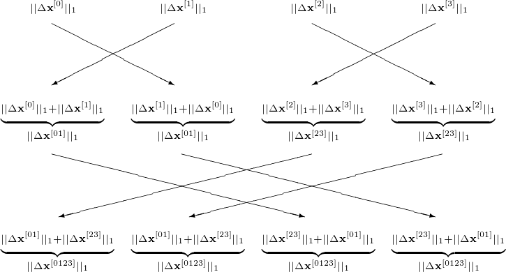
Fig. 52 Butterfly synchronization of a parallel Jacobi iteration with 4 processors.

The communication stages are as follows. At the start, every node must have \({\bf x}^{(0)}\), \(\epsilon\), \(N\), a number of rows of \(A\) and the corresponding part of the right hand side \({\bf b}\). After each update \(n/p\) elements of \({\bf x}^{(k+1)}\) must be scattered. The butterfly synchronization takes \(\log_2(p)\) steps. The scattering of \({\bf x}^{(k+1)}\) can coincide with the butterfly synchronization. The computation effort: \(O(n^2/p)\) in each stage.

A Parallel Implementation with MPI

For dimension \(n\), we consider the diagonally dominant system:

\[\begin{split}\left[ \begin{array}{cccc} n+1 & 1 & \cdots & 1 \\ 1 & n+1 & \cdots & 1 \\ \vdots & \vdots & \ddots & \vdots \\ 1 & 1 & \cdots & n+1 \\ \end{array} \right] \left[ \begin{array}{c} x_1 \\ x_2 \\ \vdots \\ x_n \end{array} \right] = \left[ \begin{array}{c} 2 n \\ 2 n \\ \vdots \\ 2 n \end{array} \right].\end{split}\]

The exact solution is \({\bf x}\): for \(i=1,2,\ldots,n\), \(x_i = 1\). We start the Jacobi iteration method at \({\bf x}^{(0)} = {\bf 0}\). The parameters are \(\epsilon = 10^{-4}\) and \(N = 2 n^2\). A session where we run the program displays on screen the following:

$ time /tmp/jacobi 1000
   0 : 1.998e+03
   1 : 1.994e+03
...
8405 : 1.000e-04
8406 : 9.982e-05
computed 8407 iterations
error : 4.986e-05

real    0m42.411s
user    0m42.377s
sys     0m0.028s

C code to run Jacobi iterations is below.

void run_jacobi_method
 ( int n, double **A, double *b, double epsilon, int maxit, int *numit, double *x );
/*
 * Runs the Jacobi method for A*x = b.
 *
 * ON ENTRY :
 *   n        the dimension of the system;
 *   A        an n-by-n matrix A[i][i] /= 0;
 *   b        an n-dimensional vector;
 *   epsilon  accuracy requirement;
 *   maxit    maximal number of iterations;
 *   x        start vector for the iteration.
 *
 * ON RETURN :
 *   numit    number of iterations used;
 *   x        approximate solution to A*x = b. */

void run_jacobi_method
 ( int n, double **A, double *b, double epsilon, int maxit, int *numit, double *x )
{
   double *dx,*y;
   dx = (double*) calloc(n,sizeof(double));
   y = (double*) calloc(n,sizeof(double));
   int i,j,k;

   for(k=0; k<maxit; k++)
   {
      double sum = 0.0;
      for(i=0; i<n; i++)
      {
         dx[i] = b[i];
         for(j=0; j<n; j++)
            dx[i] -= A[i][j]*x[j];
         dx[i] /= A[i][i];
         y[i] += dx[i];
         sum += ( (dx[i] >= 0.0) ? dx[i] : -dx[i]);
      }
      for(i=0; i<n; i++) x[i] = y[i];
      printf("%3d : %.3e\n",k,sum);
      if(sum <= epsilon) break;
   }
   *numit = k+1;
   free(dx); free(y);
}

Gather-to-All with MPI_Allgather

Gathering the four elements of a vector to four processors is schematically depicted in Fig. 53.

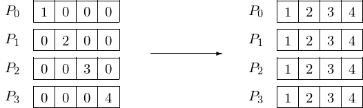
Fig. 53 Gathering 4 elements to 4 processors.

The syntax of the MPI gather-to-all command is

MPI_Allgather(sendbuf,sendcount,sendtype,
              recvbuf,recvcount,recvtype,comm)

where the parameters are in Table 18.

Table 18 The parameters of MPI_Allgather.

parameter	description
sendbuf	starting address of send buffer
sendcount	number of elements in send buffer
sendtype	data type of send buffer elements
recvbuf	address of receive buffer
recvcount	number of elements received from any process
recvtype	data type of receive buffer elements
comm	communicator

A program that implements the situation as in Fig. 53 will print the following to screen:

$ mpirun -np 4 /tmp/use_allgather
data at node 0 : 1 0 0 0
data at node 1 : 0 2 0 0
data at node 2 : 0 0 3 0
data at node 3 : 0 0 0 4
data at node 3 : 1 2 3 4
data at node 0 : 1 2 3 4
data at node 1 : 1 2 3 4
data at node 2 : 1 2 3 4
$

The code of the program use_allgather.c is below:

int i,j,p;
MPI_Init(&argc,&argv);
MPI_Comm_rank(MPI_COMM_WORLD,&i);
MPI_Comm_size(MPI_COMM_WORLD,&p);
{
   int data[p];
   for(j=0; j<p; j++) data[j] = 0;
   data[i] = i + 1;
   printf("data at node %d :",i);
   for(j=0; j<p; j++) printf(" %d",data[j]); printf("\n");
   MPI_Allgather(&data[i],1,MPI_INT,data,1,MPI_INT,MPI_COMM_WORLD);
   printf("data at node %d :",i);
   for(j=0; j<p; j++) printf(" %d",data[j]); printf("\n");
}

Applying the MPI_Allgather to a parallel version of the Jacobi method shows the following on screen:

$ time mpirun -np 10 /tmp/jacobi_mpi 1000
...
8405 : 1.000e-04
8406 : 9.982e-05
computed 8407 iterations
error : 4.986e-05

real    0m5.617s
user    0m45.711s
sys     0m0.883s

Recall that the wall clock time of the run with the sequential program equals 42.411.s. The speedup is thus 42.411/5.617 = 7.550. Code for the parallel run_jacobi_method is below.

void run_jacobi_method
 ( int id, int p, int n, double **A, double *b, double epsilon, int maxit, int *numit, double *x )
{
   double *dx,*y;
   dx = (double*) calloc(n,sizeof(double));
   y = (double*) calloc(n,sizeof(double));
   int i,j,k;
   double sum[p];
   double total;
   int dnp = n/p;
   int istart = id*dnp;
   int istop = istart + dnp;
   for(k=0; k<maxit; k++)
   {
      sum[id] = 0.0;
      for(i=istart; i<istop; i++)
      {
         dx[i] = b[i];
         for(j=0; j<n; j++)
            dx[i] -= A[i][j]*x[j];
         dx[i] /= A[i][i];
         y[i] += dx[i];
         sum[id] += ( (dx[i] >= 0.0) ? dx[i] : -dx[i]);
      }
      for(i=istart; i<istop; i++) x[i] = y[i];
      MPI_Allgather(&x[istart],dnp,MPI_DOUBLE,x,dnp,MPI_DOUBLE,MPI_COMM_WORLD);
      MPI_Allgather(&sum[id],1,MPI_DOUBLE,sum,1,MPI_DOUBLE,MPI_COMM_WORLD);
      total = 0.0;
      for(i=0; i<p; i++) total += sum[i];
      if(id == 0) printf("%3d : %.3e\n",k,total);
      if(total <= epsilon) break;
   }
   *numit = k+1;
   free(dx);
}

Let us do an analysis of the computation and communication cost. Computing \({\bf x}^{(k+1)} := {\bf x}^{(k)} + D^{-1}({\bf b} - A {\bf x}^{(k)})\) with p processors costs

\[t_{\rm comp} = \frac{n(2n + 3)}{p}.\]

We count \(2n + 3\) operations because of

• one \(-\) and one \(\star\) when running over the columns of \(A\); and
• one \(/\), one \(+\) for the update and one \(+\) for the \(||\cdot||_1\).

The communication cost is

\[t_{\rm comm} = p \left(t_{\rm startup} + \frac{n}{p} t_{\rm data} \right).\]

In the examples, the time unit is the cost of one arithmetical operation. Then the costs \(t_{\rm startup}\) and \(t_{\rm data}\) are multiples of this unit.

Finding the p with the minimum total cost is illustrated in Fig. 54 and Fig. 55.

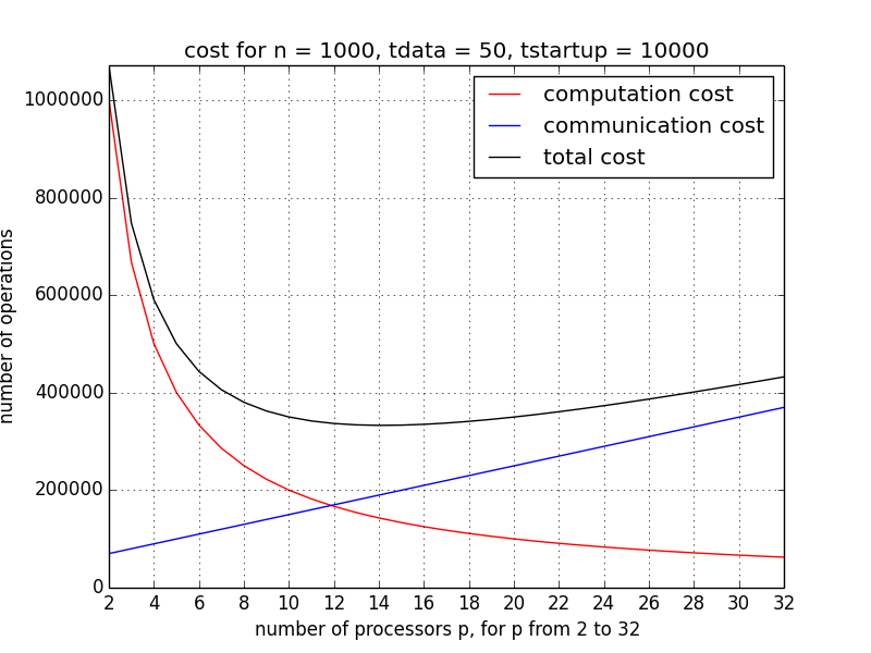
Fig. 54 With increasing p, the (red) computation cost decreases, while the (blue) communication cost increases. The minimum of the (black) total cost is the optimal value for p.

In Fig. 54, the communication, computation, and total cost is shown for p ranging from 2 to 32, for one iteration, with \(n = 1,000\), \(t_{\rm startup} = 10,000\), and \(t_{\rm data} = 50\). We see that the total cost starts to increase once p becomes larger than 16. For a larger dimension, after a ten-fold increase, \(n = 10,000\), \(t_{\rm startup} = 10,000\), and \(t_{\rm data} = 50\), the scalability improves, as in Fig. 55, p ranges from 16 to 256.

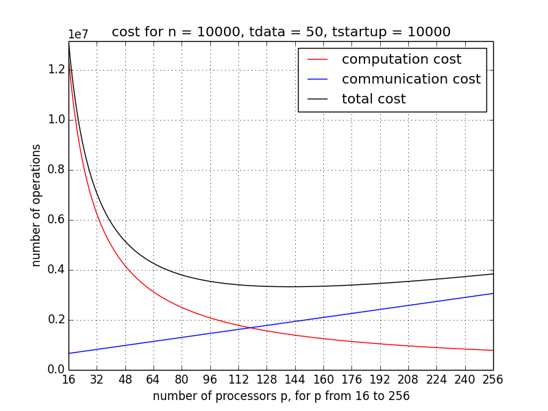
Fig. 55 With increasing p, the (red) computation cost decreases, while the (blue) communication cost increases. The minimum of the (black) total cost is the optimal value for p.

Exercises

1. Use OpenMP to write a parallel version of the Jacobi method. Do you observe a better speedup than with MPI?
2. The power method to compute the largest eigenvalue of a matrix A uses the formulas \({\bf y} := A {\bf x}^{(k)}\); \({\bf x}^{(k+1)} := {\bf y}/||{\bf y}||\). Describe a parallel implementation of the power method.
3. Consider the formula for the total cost of the Jacobi method for an n-dimensional linear system with p processors. Derive an analytic expression for the optimal value of p. What does this expression tell about the scalability?