Performance Considerations

Our goal is to fully occupy the GPU. When launching a kernel, we set the number of blocks and number of threads per block. For full occupancy, we want to reach the largest number of resident blocks and threads. The number of threads ready for execution may be limited by constraints on the number of registers and shared memory.

Dynamic Partitioning of Resources

In Table 28 we compare the compute capabilities of a Streaming Multiprocessor (SM) for the graphics cards with respective compute capabilities 1.1, 2.0, 3.5, and 6.0: GeForce 9400M, Tesla C2050/C2070, K20C, and P100.

Table 28 Compute Capabilities 1.1, 2.0, 3.5, 6.0.

compute capability	1.1	2.0	3.5	6.0
maximum number of threads per block	512	1,024	1,024	1,024
maximum number of blocks per SM	8	8	16	32
warp size	32	32	32	32
maximum number of warps per SM	24	48	64	64
maximum number of threads per SM	768	1,536	2,048	2,048

During runtime, thread slots are partitioned and assigned to thread blocks. Streaming multiprocessors are versatile by their ability to dynamically partition the thread slots among thread blocks. They can either execute many thread blocks of few threads each, or execute a few thread blocks of many threads each. In contrast, fixed partitioning where the number of blocks and threads per block are fixed will lead to waste.

We consider the interactions between resource limitations on the C2050. The Tesla C2050/C2070 has 1,536 thread slots per streaming multiprocessor. As \(1,536 = 32 \times 48\), we have

\[\mbox{number of thread slots } = \mbox{warp size } \times \mbox{ number of warps per block.}\]

For 32 threads per block, we have 1,536/32 = 48 blocks. However, we can have at most 8 blocks per streaming multiprocessor. Therefore, to fully utilize both the block and thread slots, to have 8 blocks, we should have

• \(1,536/8 = 192\) threads per block, or
• \(192/32 = 6\) warps per block.

On the K20C, the interaction between resource liminations differ. The K20C has 2,048 thread slots per streaming multiprocessor. The total number of thread slots equals \(2,048 = 32 \times 64\). For 32 threads per block, we have 2,048/32 = 64 blocks. However, we can have at most 16 blocks per streaming multiprocessor. Therefore, to fully utilize both the block and thread slots, to have 16 blocks, we should have

• \(2,048/16 = 128\) threads per block, or
• \(128/32 = 4\) warps per block.

On the P100, there is another slight difference in the resource limitation, which leads to another outcome. In particular, we now can have at most 32 blocks per streaming multiprocessor. To have 32 blocks, we should have

• \(2,048/32 = 64\) threads per block, or
• \(64/32 = 2\) warps per block.

The memory resources of a streaming multiprocessor are compared in Table 29, for the graphics cards with respective compute capabilities 1.1, 2.0, 3.5, and 6.0: GeForce 9400M, Tesla C2050/C2070, K20C, and P100.

Table 29 memory resources for several compute capabilities.

compute capability	1.1	2.0	3.5	6.0
number of 32-bit registers per SM	8K	32KB	64KB	64KB
maximum amount of shared memory per SM	16KB	48KB	48KB	64KB
number of shared memory banks	16	32	32	32
amount of local memory per thread	16KB	512KB	512KB	512KB
constant memory size	64KB	64KB	64KB	64KB
cache working set for constant memory per SM	8KB	8KB	8KB	10KB

Local memory resides in device memory, so local memory accesses have the same high latency and low bandwidth as global memory.

Registers hold frequently used programmer and compiler-generated variables to reduce access latency and conserve memory bandwidth. Variables in a kernel that are not arrays are automatically placed into registers.

By dynamically partitioning the registers among blocks, a streaming multiprocessor can accommodate more blocks if they require few registers, and fewer blocks if they require many registers. As with block and thread slots, there is a potential interaction between register limitations and other resource limitations.

Consider the matrix-matrix multiplication example. Assume

• the kernel uses 21 registers, and
• we have 16-by-16 thread blocks.

How many threads can run on each streaming multiprocessor?

1. We calculate the number of registers for each block: \(16 \times 16 \times 21 = 5,376\) registers.
2. We have \(32 \times 1,024\) registers per SM: \(32 \times 1,024/5,376 = 6\) blocks; and \(6 < 8 =\) the maximum number of blocks per SM.
3. We calculate the number of threads per SM: \(16 \times 16 \times 6 = 1,536\) threads; and we can have at most 1,536 threads per SM.

We now introduce the performance cliff, assuming a slight increase in one resource. Suppose we use one extra register, 22 instead of 21. To answer how many threads now can run on each SM, we follow the same calculations.

1. We calculate the number of registers for each block: \(16 \times 16 \times 22 = 5,632\) registers.
2. We have \(32 \times 1,024\) registers per SM: \(32 \times 1,024/5,632 = 5\) blocks.
3. We calculate the number of threads per SM: \(16 \times 16 \times 5 = 1,280\) threads; and with 21 registers we could use all 1,536 threads per SM.

Adding one register led to a reduction of 17% in the parallelism.

Definition of performance cliff

When a slight increase in one resource leads to a dramatic reduction in parallelism and performance, one speaks of a performance cliff.

The CUDA compiler tool set contains a spreadsheet to compute the occupancy of the GPU, as shown in Fig. 113.

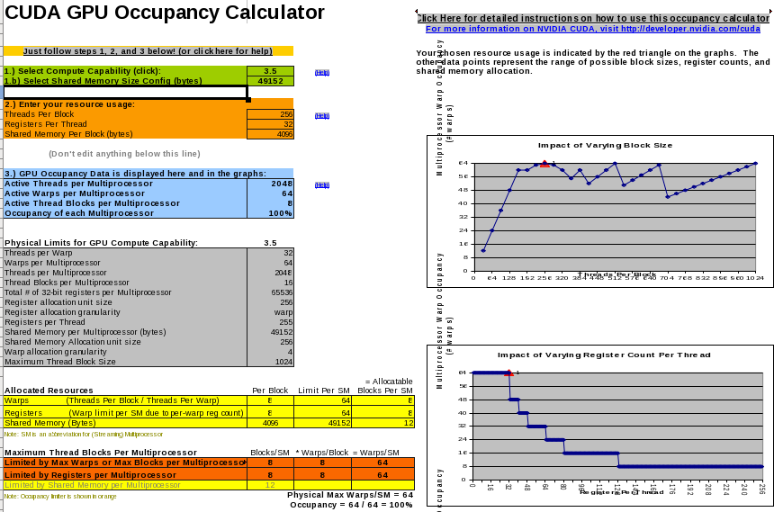
Fig. 113 The CUDA occupancy calculator.

The Compute Visual Profiler

The Compute Visual Profiler is a graphical user interface based profiling tool to measure performance and to find potential opportunities for optimization in order to achieve maximum performance.

We look at one of the example projects matrixMul. The analysis of the kernel matrixMul is displayed in Fig. 114, Fig. 115, Fig. 116, Fig. 117, and Fig. 118.

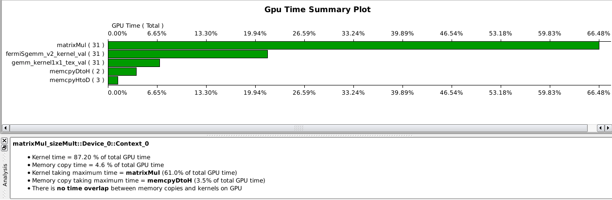
Fig. 114 GPU time summary of the matrixMul kernel.

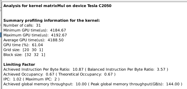
Fig. 115 Limiting factor identification of the matrixMul kernel, IPC = Instructions Per Cycle.

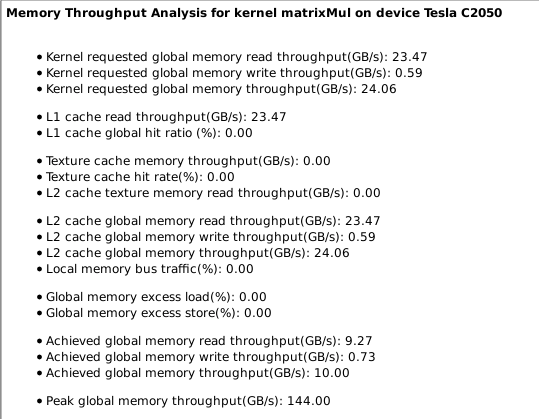
Fig. 116 Memory throughput analysis of the matrixMul kernel.

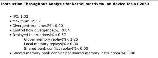
Fig. 117 Instruction throughput analysis of the matrixMul kernel, IPC = Instructions Per Cycle.

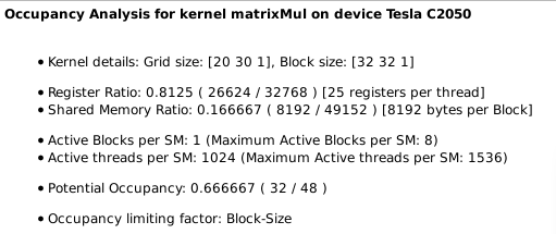
Fig. 118 Occupancy analysis of the matrixMul kernel.

Data Prefetching and Instruction Mix

One of the most important resource limitations is access to global memory and long latencies. Scheduling other warps while waiting for memory access is powerful, but often not enough. A complementary to warp scheduling solution is to prefetch the next data elements while processing the current data elements. Combined with tiling, data prefetching provides extra independent instructions to enable the scheduling of more warps to tolerate long memory access latencies.

For the tiled matrix-matrix multiplication, the pseudo code below combines prefetching with tiling:

load first tile from global memory into registers;
loop
{
   deposit tile from registers to shared memory;
   __syncthreads();
   load next tile from global memory into registers;
   process current tile;
   __syncthreads();
}

The prefetching adds independent instructions between loading the data from global memory and processing the data.

Table Table 30 is taken from Table 2 of the CUDA C Programming Guide. The ftp in Table 30 stands for floating-point and int for integer.

Table 30 Number of operations per clock cycle per multiprocessor.

compute capability	1.x	2.0	3.5	6.0
32-bit fpt add, multiply, multiply-add	8	32	192	64
64-bit fpt add, multiply, multiply-add	1	16	64	4
32-bit int add, logical operation, shift, compare	8	32	160	128
32-bit fpt reciprocal, sqrt, log, exp, sin, cos	2	4	32	32

Consider the following code snippet:

for(int k = 0; k < m; k++)
   C[i][j] += A[i][k]*B[k][j];

Counting all instructions:

• 1 loop branch instruction (k < m);
• 1 loop counter update instruction (k++);
• 3 address arithmetic instructions ([i][j], [i][k], [k][j]);
• 2 floating-point arithmetic instructions (+ and *).

Of the 7 instructions, only 2 are floating point.

Loop unrolling reduces the number of loop branch instructions, loop counter updates, address arithmetic instructions. Note: gcc -funroll-loops is enabled with gcc -O2.

Exercises

1. Examine the occupancy calculator for the graphics card on your laptop or desktop.
2. Read the user guide of the compute visual profiler and perform a run on GPU code you wrote (of some previous exercise or your code for the third project). Explain the analysis of the kernel.
3. Redo the first interactions between resource limitations of this lecture using the specifications for compute capability 1.1.
4. Redo the second interactions between resource limitations of this lecture using the specifications for compute capability 1.1.