L-20 MCS 572 Friday 24 February 2005
| > | restart; |
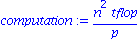
This Maple worksheet provides a model to evaluate the optimal number of processors for a plain parallel Jacobi iteration on a dense matrix of dimension n, for p processors. The other parameters in the model are the time to do a floating-point operation (denoted by tflop) and the times to send/receive one data element and to startup the communications (respectively denoted by tdata and tstartup).
Here are the formulas:
| > | computation := n^2*tflop/p; |
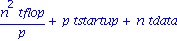
| > | communication := p*tstartup + n*tdata; |

| > | total := computation + communication; |

Because it is interesting to plot the these three formulas for various values of the parameters, we put the plotting commands in a procedure:
| > | speedup_plot := proc(n,tflop,tdata,tstartup,pmin,pmax)
description `shows the speedup plot for problem of size n, using tflop, tdata, and tstartup as respective times for one flop, to send one data element, and to start up the communications, for range of processors between pmin and pmax`: local computation,communication,total,p,plotcomp,plotcomm,plottotal: computation := n^2*tflop/p: communication := p*tstartup + n*tdata: total := computation + communication: plotcomp := plot(computation,p=pmin..pmax,color=green): plotcomm := plot(communication,p=pmin..pmax,color=blue): plottotal := plot(total,p=pmin..pmax,color=red): plots[display](plotcomp,plotcomm,plottotal); end proc: |
Just watch if we take some "typical" values for tflop, tdata, and tstartup, for varying values of n:
| > | speedup_plot(1000,1,50,20000,2,20); |
![[Plot]](images/speedup_jacobi_4.gif)
| > | speedup_plot(2000,1,50,20000,2,20); |
![[Plot]](images/speedup_jacobi_5.gif)
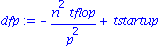
We see the optimal number of processors increase as the problem size n doubles. We just have to solve a general quadratic formula to find the optimal number of processors:
| > | total; |
| > | dfp := diff(total,p); |
| > | sol := solve(dfp,p); |

| > | opt_np := (N,f,s) -> subs(n=N,tstartup=s,tflop=f,abs(sol[1])); |
![opt_np := proc (N, f, s) options operator, arrow; subs(n = N, tstartup = s, tflop = f, abs(sol[1])) end proc](images/speedup_jacobi_9.gif)
| > | opt_np(1000,1,20000); evalf(%); |


| > | opt_np(2000,1,20000); evalf(%); |


| > | plot(opt_np(n,1,20000),n=1000..100000); |
![[Plot]](images/speedup_jacobi_14.gif)
| > |
The plot confirms that the optimal number of processors is linear in n.