Tasking with OpenMP¶

A process can be viewed as a program. A process can have multiple threads of execution.

Tasks are much lighter than threads. The main differences between threads and tasks are:

Starting and terminating a task is much faster than starting and terminating a thread.
A thread has its own process id and own resources, whereas a task is typically a small routine.

Parallel Recursive Functions¶

The sequence of Fibonacci numbers $F_n$ are defined as

\[F_0 = 0, \quad F_1 = 1, \quad \mbox{and for } n>1: F_n = F_{n-1} + F_{n-2}.\]

This leads to a natural recursive function.

The recursion generates many function calls. While inefficient to compute $F_n$, this recursion serves as a parallel pattern.

The parallel version is part of the OpenMP Application Programming Interface Examples. The Fibonacci function with tasking demonstrates the generation of a large number of tasks with one thread. No parallelism will result from this example.

But it is instructive to introduce basic task constructs.

The task construct defines an explicit task.
The taskwait construct synchronizes sibling tasks.
The shared clause of a task construct declares a variable to be shared by tasks.

The start of the program takes the number of threads as a command line argument, or, when that number is omitted, prompts the user for the number of threads:

#include <stdio.h>
#include <stdlib.h>
#include <omp.h>

int fib ( int n );
/* Returns the n-th Fibonacci number,
 * computed recursively with tasking. */

int main ( int argc, char *argv[] )
{
   int n;

   if(argc > 1)
      n = atoi(argv[1]);
   else
   {
      printf("Give n : "); scanf("%d", &n);
   }
   omp_set_num_threads(8);

   #pragma omp parallel
   {
      #pragma omp single
      printf("F(%d) = %d\n",n,fib(n));
   }
   return 0;
}

The single construct specifies that the statement is executed by only one thread in the team. In this example, one thread generates many tasks. The definition of a parallel recursive Fibonacci function is below.

int fib ( int n )
{
   if(n < 2)
      return n;
   else
   {
      int left,right;    // shared by all tasks

      #pragma omp task shared(left)
      left = fib(n-1);

      #pragma omp task shared(right)
      right = fib(n-2);
                           // synchronize tasks
      #pragma omp taskwait
      return left + right;
   }
}

Parallel Recursive Quadrature¶

The recursive parallel computation of the Fibonacci number serves as a pattern to compute integrals by recursively dividing the integration interval.

Let us apply a numerical integration rule $R(f,a,b,n)$ to $\displaystyle \int_a^b f(x) dx$. The rule $R(f,a,b,n)$ takes on input

the function $f$, bounds $a$, $b$ of $[a,b]$, and
the number $n$ of function evaluations.

The rule returns and approximation $A$ and an error estimate $e$.

If $e$ is larger than some tolerance, then

$c = (b-a)/2$ is the middle of $[a,b]$,
compute $A_1, e_1 = R(f,a,c,n)$,
compute $A_2, e_2 = R(f,c,a,n)$,
return $A_1 + A_2, e_1 + e_2$.

As a rule, the composite trapezoidal rule is applied recursively. Using $n$ subintervals of $[a,b]$, the rule is

\[R(f,a,b,n) = \frac{h}{2}(f(a) + f(b)) + h \sum_{i=1}^{n-1} f(a + ih), \quad h = \frac{b-a}{n}.\]

In our setup, let $f(x) = e^x$, $[a,b] = [0,1]$, then $\displaystyle \int_0^1 e^x dx = e - 1$.

We keep $n$ fixed. Let $d$ be the depth of the recursion. The recursion level is $\ell$. Pseudo code is below.

${\cal F}(\ell, d, f, a, b, n)$:

If $\ell = d$ then
return $R(f,a,b,n)$
else
$c = (b-a)/2$
return ${\cal F}(\ell\!+\!1,d,f,a,c,n) + {\cal F}(\ell\!+\!1,d,f,c,b,n)$.

The tree of function calls is shown in Fig. 37. The root of the tree is the first call, omitting the value for $n$, the number of function calls.

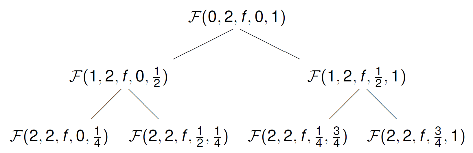
_images/figrecursivequadrature.png — Fig. 37 A tree of recursive function calls of depth 2.¶

At the leaves of the tree, the rule is applied. As all computations are concentrated at the leaves, we expect speedups from a parallel execution.

A recursive parallel integration function with OpenMP is defined below.

double rectraprule
 ( int level, int depth,
   double (*f) ( double x ), double a, double b, int n )
{
   if(level == depth)
      return traprule(f,a,b,n);
   else
   {
      double middle = (b - a)/2;
      double left,right;

      #pragma omp task shared(left)
      left = rectraprule(level+1,depth,f,a,middle,n);

      #pragma omp task shared(right)
      right = rectraprule(level+1,depth,f,middle,b,n);

      #pragma omp taskwait
      return left + right;
   }
}

Timing the running with 8 threads is shown below.

$ time ./comptraprec 200000 10
approximation = 1.7182818284620265e+00
   exp(1) - 1 = 1.7182818284590451e+00, error = 2.98e-12

real    0m3.299s
user    0m3.298s
sys     0m0.001s
$ time ./comptraprecomp 200000 10
approximation = 1.7182818284620265e+00
   exp(1) - 1 = 1.7182818284590451e+00, error = 2.98e-12

real    0m0.743s
user    0m4.003s
sys     0m0.004s
$

Observe the speedup, when comparing the wall clock times (real).

Bernstein’s Conditions¶

Given a program, which statements can be executed in parallel? Let us do a dependency analysis.

Let $u$ be an operation. Denote:

${\cal R}(u)$ is the set of memory cells $u$ reads,
${\cal M}(u)$ is the set of memory cells $u$ modifies.

Two operations $u$ and $v$ are independent if

${\cal M}(u) \cap {\cal M}(v) = \emptyset$, and
${\cal M}(u) \cap {\cal R}(v) = \emptyset$, and
${\cal R}(u) \cap {\cal M}(v) = \emptyset.$

The above conditions are known as Bernstein’s conditions. Checking Bernstein’s conditions is easy for operations on scalars, is more difficult for array accesses, and is almost impossible for pointer dereferencing.

As an example, let x be some scalar and consider two statements:

$u$: x = x + 1,
$v$: x = x + 2.

We see that $u$ and $v$ are independent of each other, because $u$ followed by $v$ or $v`$ followed by $u$ is equivalent to

\[w\!: \mbox{\tt x = x + 3}.\]

However, execution of $u$ and $v$ happens by a sequence of more elementary instructions:

$u$: r1 = x; r1 += 1; x = r1;
$v$: r2 = x; r2 += 2; x = r2;

where r1 and r2 are registers. The elementary instructions are no longer independent.

Task Dependencies¶

With the depend clause of OpenMP, the order of execution of tasks can be ordered.

In the depend clause, we consider two dependence types:

The in type: the task depends on the sibling task(s) that generates the item followed by the in:.
The out type: if an item appeared following an in: then there should be task with the clause `` out``.

The code below is copied from the OpenMP API Examples section.

#include <stdio.h>
#include <omp.h}

int main ( int argc, char *argv[] )
{
   int x = 1;

   #pragma omp parallel
   #pragma omp single
   {
       #pragma omp task shared(x) depend(out: x)
       x = 2;
       #pragma omp task shared(x) depend(in: x)
       printf("x = %d\n", x);
   }
   return 0;
}

In the parallel region, the single construct indicates that every instruction needs to be execute only once.

One task assigns 2 to x.
Another task prints the value of x.

Without depend, tasks could execute in any order, and the program would have a race condition.

The depend clauses force the ordering of the tasks. The example always prints x = 2.

Parallel Blocked Matrix Multiplication¶

Our last example also comes from the OpenMP API Examples. Consider the product of two blocked matrices $A$ with $B$:

\[\begin{split}\left[ \begin{array}{cc} A_{1,1} & A_{1,2} \\ A_{2,1} & A_{2,2} \end{array} \right] \left[ \begin{array}{cc} B_{1,1} & B_{1,2} \\ B_{2,1} & B_{2,2} \end{array} \right] = \left[ \begin{array}{cc} C_{1,1} & C_{1,2} \\ C_{2,1} & C_{2,2} \end{array} \right].\end{split}\]

where

\[C_{i,j} = A_{i,1} B_{1,j} + A_{i,2} B_{2,j},\]

for all $i$ and $j$. The arguments of the depend clauses are blocked matrices.

Matrices are stored as pointers to rows. Allocating a matrix of dimension dim:

double **A;
int i;

A = (double**)calloc(dim, sizeof(double*));

for(i=0; i<dim; i++) A[i] = (double*)calloc(dim, sizeof(double));

Every row A[i] is allocated in the loop.

We consider multiplying blocked matrices of random doubles. At the command line, we specify

the block size, the size of each block,
the number of blocks in every matrix, and
the number of threads.

The dimension equals the block size times the number of blocks.

The parallel region:

#pragma omp parallel
#pragma omp single
matmatmul(dim,blocksize,A,B,C);

One single thread calls the function matmatmul. The matmatmul generates a large number of tasks. The function matmatmul begins as

void matmatmul
 ( int N, int BS,
   double **A, double **B, double **C )
{
   int i, j, k, ii, jj, kk;

   for(i=0; i<N; i+=BS)
   {
      for(j=0; j<N; j+=BS)
      {
         for(k=0; k<N; k+=BS)
         {

The triple loop computes the block $C_{i,j}$.

Each task has its own indices ii, jj, and kk.

#pragma omp task private(ii, jj, kk) \
        depend(in: A[i:BS][k:BS], B[k:BS][j:BS]) \
        depend(inout: C[i:BS][j:BS])
{
   for(ii=i; ii<i+BS; ii++)
      for(jj=j; jj<j+BS; jj++)
         for(kk=k; kk<k+BS; kk++)
            C[ii][jj] = C[ii][jj] + A[ii][kk]*B[kk][jj];
}

The inout dependence type C[i:BS][j:BS] expresses that the dependencies of the update of the block $C_{i,j}$.

Runs with 2 and 4 threads are shown below.

$ gcc -fopenmp -O3 -o matmulomp matmulomp.c

$ time ./matmulomp 500 2 2

real    0m0.828s
user    0m1.558s
sys     0m0.020s

$ time ./matmulomp 500 2 4

real    0m0.445s
user    0m1.575s
sys     0m0.017s
$

PLASMA (Parallel Linear Algebra Software for Multicore Architectures) is a numerical library intended as a successor to LAPACK for solving problems in dense linear algebra on multicore processors. As indicated in the bibliography section, the PLASMA developers used the OpenMP standard.

Bibliography¶

A. J. Bernstein: Analysis of Programs for Parallel Processing. IEEE Transactions on Electronic Computers 15(5):757-763, 1966.
P. Feautrier: Bernstein’s Conditions. In Encycopedia of Parallel Computing, edited by David Padua, pages 130-133, Springer 2011.
C. von Praun: Race Conditions. In Encycopedia of Parallel Computing, edited by David Padua, pages 1691-1697, Springer 2011.
B. Wilkinson and M. Allen: Parallel Programming. Techniques and Applications Using Networked Workstations and Parallel Computers. 2nd Edition. Prentice-Hall 2005.
A. YarKhan, J. Kurzak, P. Luszczek, J. Dongarra: Porting the PLASMA Numerical Library to the OpenMP Standard. International Journal of Parallel Programming, May 2016.

Exercises¶

Label the six elementary operations in the example on the Bernstein’s conditions as $u_1$, $u_2$, $u_3$, $v_1$, $v_2$, $v_3$.

Write for each the sets ${\cal R}(\cdot)$ and ${\cal M}(\cdot)$.

Based on the dependency analysis, arrange the six instructions for a correct parallel computation.
The block size, number of blocks, and number of threads are the three parameters in matmulomp.

Explore experimentally with matmulomp the relationship between the number of blocks and the number of threads.

For which values do you obtain a good speedup?

Tasking with OpenMP¶

Parallel Recursive Functions¶

Parallel Recursive Quadrature¶

Bernstein’s Conditions¶

Task Dependencies¶

Parallel Blocked Matrix Multiplication¶

Bibliography¶

Exercises¶

Table of Contents

Previous topic

Next topic

This Page