Data Parallelism and Matrix Multiplication
Matrix multiplication is one of the fundamental building blocks in numerical linear algebra, and therefore in scientific computation. In this section, we investigate how data parallelism may be applied to solve this problem.
Data Parallelism
Many applications process large amounts of data. Data parallelism refers to the property where many arithmetic operations can be safely performed on the data simultaneously. Consider the multiplication of matrices \(A\) and \(B\) which results in \(C = A \cdot B\), with
\(c_{i,j}\) is the inner product of the i-th row of \(A\) with the j-th column of \(B\):
All \(c_{i,j}\)’s can be computed independently from each other. For \(n = m = p = 1,024\) we have 1,048,576 inner products. The matrix multiplication is illustrated in Fig. 56.
Code for Matrix-Matrix Multiplication
Code for a device (the GPU) is defined in functions
using the keyword __global__ before the function definition.
Data parallel functions are called kernels.
Kernel functions generate a large number of threads.
In matrix-matrix multiplication, the computation can be implemented as a kernel where each thread computes one element in the result matrix. To multiply two 1,000-by-1,000 matrices, the kernel using one thread to compute one element generates 1,000,000 threads when invoked.
CUDA threads are much lighter weight than CPU threads: they take very few cycles to generate and schedule thanks to efficient hardware support whereas CPU threads may require thousands of cycles.
A CUDA program consists of several phases, executed on
the host: if no data parallelism, or
on the device: for data parallel algorithms.
The NVIDIA C compiler nvcc separates phases at compilation.
Code for the host is compiled on host’s standard C compilers
and runs as ordinary CPU process.
device code is written in C with keywords for data parallel
functions and further compiled by nvcc.
A CUDA program has the following structure:
CPU code
kernel<<<numb_blocks,numb_threads_per_block>>>(args)
CPU code
The number of blocks in a grid is illustrated in Fig. 63.
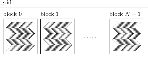
Fig. 63 The organization of the threads of execution in a CUDA program.
For the matrix multiplication \(C = A \cdot B\), we run through the following stages:
Allocate device memory for \(A\), \(B\), and \(C\).
Copy \(A\) and \(B\) from the host to the device.
Invoke the kernel to have device do \(C = A \cdot B\).
Copy \(C\) from the device to the host.
Free memory space on the device.
A linear address system is used for the 2-dimensional array. Consider a 3-by-5 matrix stored row-wise (as in C), as shown in Fig. 58. Code to generate a random matrix is below:
#include <stdlib.h>

__host__ void randomMatrix ( int n, int m, float *x, int mode )
/*
 * Fills up the n-by-m matrix x with random
 * values of zeroes and ones if mode == 1,
 * or random floats if mode == 0. */
{
   int i,j,r;
   float *p = x;

   for(i=0; i<n; i++)
      for(j=0; j<m; j++)
      {
         if(mode == 1)
            r = rand() % 2;
         else
            r = ((float) rand())/RAND_MAX;
         *(p++) = (float) r;
      }
}
The writing of a matrix is defined by the following code:
#include <stdio.h>

__host__ void writeMatrix ( int n, int m, float *x )
/*
 * Writes the n-by-m matrix x to screen. */
{
   int i,j;
   float *p = x;

   for(i=0; i<n; i++,printf("\n"))
      for(j=0; j<m; j++)
         printf(" %d", (int)*(p++));
}
In defining the kernel, we assign inner products to threads.
For example, consider a 3-by-4 matrix \(A\)
and a 4-by-5 matrix \(B\), as in Fig. 59.
The i = blockIdx.x*blockDim.x + threadIdx.x
determines what entry in \(C = A \cdot B\) will be computed:
the row index in \(C\) is
idivided by 5 andthe column index in \(C\) is the remainder of
idivided by 5.
The kernel function is defined below:
__global__ void matrixMultiply
 ( int n, int m, int p, float *A, float *B, float *C )
/*
 * Multiplies the n-by-m matrix A
 * with the m-by-p matrix B into the matrix C.
 * The i-th thread computes the i-th element of C. */
{
   int i = blockIdx.x*blockDim.x + threadIdx.x;
   C[i] = 0.0;
   int rowC = i/p;
   int colC = i%p;
   float *pA = &A[rowC*m];
   float *pB = &B[colC];
   for(int k=0; k<m; k++)
   {
      pB = &B[colC+k*p];
      C[i] += (*(pA++))*(*pB);
   }
}
Running the program in a terminal window is shown below.
$ /tmp/matmatmul 3 4 5 1
a random 3-by-4 0/1 matrix A :
 1 0 1 1
 1 1 1 1
 1 0 1 0
a random 4-by-5 0/1 matrix B :
 0 1 0 0 1
 0 1 1 0 0
 1 1 0 0 0
 1 1 0 1 0
the resulting 3-by-5 matrix C :
 2 3 0 1 1
 2 4 1 1 1
 1 2 0 0 1
$
The main program takes four command line arguments: the dimensions of the matrices, that is: the number of rows and columns of \(A\), and the number of columns of \(B\). The fourth element is the mode, whether output is needed or not. The parsing of the command line arguments is below:
int main ( int argc, char*argv[] )
{
   if(argc < 4)
   {
      printf("Call with 4 arguments :\n");
      printf("dimensions n, m, p, and the mode.\n");
   }
   else
   {
      int n = atoi(argv[1]);    /* number of rows of A */
      int m = atoi(argv[2]);    /* number of columns of A */
                                /* and number of rows of B */
      int p = atoi(argv[3]);    /* number of columns of B */
      int mode = atoi(argv[4]); /* 0 no output, 1 show output */
      if(mode == 0)
         srand(20140331)
      else
         srand(time(0));
The next stage in the main program is the allocation of memories, on the host and on the device, as listed below:
float *Ahost = (float*)calloc(n*m,sizeof(float));
float *Bhost = (float*)calloc(m*p,sizeof(float));
float *Chost = (float*)calloc(n*p,sizeof(float));
randomMatrix(n,m,Ahost,mode);
randomMatrix(m,p,Bhost,mode);
if(mode == 1)
{
   printf("a random %d-by-%d 0/1 matrix A :\n",n,m);
   writeMatrix(n,m,Ahost);
   printf("a random %d-by-%d 0/1 matrix B :\n",m,p);
   writeMatrix(m,p,Bhost);
}
/* allocate memory on the device for A, B, and C */
float *Adevice;
size_t sA = n*m*sizeof(float);
cudaMalloc((void**)&Adevice,sA);
float *Bdevice;
size_t sB = m*p*sizeof(float);
cudaMalloc((void**)&Bdevice,sB);
float *Cdevice;
size_t sC = n*p*sizeof(float);
cudaMalloc((void**)&Cdevice,sC);
After memory allocation, the data is copied from host to device and the kernels are launched.
/* copy matrices A and B from host to the device */
cudaMemcpy(Adevice,Ahost,sA,cudaMemcpyHostToDevice);
cudaMemcpy(Bdevice,Bhost,sB,cudaMemcpyHostToDevice);

/* kernel invocation launching n*p threads */
matrixMultiply<<<n*p,1>>>(n,m,p,
                          Adevice,Bdevice,Cdevice);

/* copy matrix C from device to the host */
cudaMemcpy(Chost,Cdevice,sC,cudaMemcpyDeviceToHost);
/* freeing memory on the device */
cudaFree(Adevice); cudaFree(Bdevice); cudaFree(Cdevice);
if(mode == 1)
{
   printf("the resulting %d-by-%d matrix C :\n",n,p);
   writeMatrix(n,p,Chost);
}
Two Dimensional Arrays of Threads
Using threadIdx.x and threadIdx.y
instead of a one dimensional organization of the threads in a block
we can make the \((i,j)\)-th thread compute \(c_{i,j}\).
The main program is then changed into
/* kernel invocation launching n*p threads */
dim3 dimGrid(1,1);
dim3 dimBlock(n,p);
matrixMultiply<<<dimGrid,dimBlock>>>
   (n,m,p,Adevice,Bdevice,Cdevice);
The above construction creates a grid of one block. The block has \(n \times p\) threads:
threadIdx.xwill range between 0 and \(n-1\), andthreadIdx.ywill range between 0 and \(p-1\).
The new kernel is then:
__global__ void matrixMultiply
 ( int n, int m, int p, float *A, float *B, float *C )
/*
 * Multiplies the n-by-m matrix A
 * with the m-by-p matrix B into the matrix C.
 * The (i,j)-th thread computes the (i,j)-th element of C. */
{
   int i = threadIdx.x;
   int j = threadIdx.y;
   int ell = i*p + j;
   C[ell] = 0.0;
   float *pB;
   for(int k=0; k<m; k++)
   {
      pB = &B[j+k*p];
      C[ell] += A[i*m+k]*(*pB);
   }
}
Examining Performance
Performance is often expressed in terms of flops.
1 flops = one floating-point operation per second;
use
perf: Performance analysis tools for Linuxrun the executable, with
perf statperf stat ./matmatmul0 1024 1024 1024 0
with the events following the
-eflag we count the floating-point operations.perf stat -e fp_arith_inst_retired.scalar_single \ ./matmatmul0 1024 1024 1024 0
Executables are compiled with the option -O2.
Running on one Intel Xeon E5-2699v4 Broadwell core, the output is listed below:
$ perf stat -e fp_arith_inst_retired.scalar_single \
  ./matmatmul0 768 768 768 0

 Performance counter stats for './matmatmul0 768 768 768 0':

       905,969,664      fp_arith_inst_retired.scalar_single:u

       1.039681742 seconds time elapsed

       1.036818000 seconds user
       0.002999000 seconds sys
Did 905,969,664 operations in 1.037 seconds:
Let us compared this run with the P100:
$ perf stat -e fp_arith_inst_retired.scalar_single
  ./matmatmul1 768 768 768 0

 Performance counter stats for './matmatmul1 768 768 768 0':

             6,123      fp_arith_inst_retired.scalar_single:u

       0.207871212 seconds time elapsed

       0.039441000 seconds user
       0.167880000 seconds sys
The drop from 1.037 seconds to 0.28 seconds is not impressive. The dimension 768 is too small for the GPU to be able to improve much. Let us run this on larger dimensions. First on the CPU:
$ perf stat -e fp_arith_inst_retired.scalar_single
  ./matmatmul0 4096 4096 4096 0

 Performance counter stats for './matmatmul0 4096 4096 4096 0':

   137,438,953,472      fp_arith_inst_retired.scalar_single:u

     416.494934403 seconds time elapsed

     416.466205000 seconds user
       0.047003000 seconds sys
and then on the GPU:
$ perf stat ./matmatmul1 4096 4096 4096 0
which shows 0.569705088 seconds time elapsed.
The speedup is 416.495/0.570 = 730, which is significant. Counting flops, f = 137,438,953,472, the performance is
\(t_{\rm cpu} = 415.495\) and \(f/t_{\rm cpu}/(2^{30}) = 0.3\) GFlops.
\(t_{\rm gpu} = 0.570\) and \(f/t_{\rm gpu}/(2^{30}) = 224.5\) GFlops.
The performance is far from optimal, both for CPU and GPU. Therefore, we will examine improved versions in the next lectures.
using CUDA.jl and Metal.jl
A plain matrix matrix multiplication in Julia
with CUDA.jl is listed below:
using CUDA

function matmul!(C, A, B)
    i = threadIdx().x
    j = threadIdx().y
    for k=1:size(A, 2)
        @inbounds C[i, j] = C[i, j] + A[i, k]*B[k, j]
    end
end

dim = 2^2
A_h = rand(dim, dim)
B_h = rand(dim, dim)
C_h = A_h * B_h
A_d = CuArray(A_h)
B_d = CuArray(B_h)
C_d = CuArray(zeros(dim, dim))

@cuda threads=(dim, dim) matmul!(C_d, A_d, B_d)

println(C_h)
println(C_d)
On a macOS GPU using Apple’s Metal framework,
the equivalent code uses Metal.jl, listed below.
using Metal

function matmul!(C, A, B)
    threadpos = thread_position_in_grid_2d()
    i = threadpos[1]
    j = threadpos[2]
    for k=1:size(A, 2)
        @inbounds C[i, j] = C[i, j] + A[i, k]*B[k, j]
    end
end
Observe the threadpos to work
with the two dimensional grid of threads.
The code continues below.
Because the GPU in an M1 MacBook Air does not support 64-bit floats,
we use Float32 instead of the default Float64:
dim = 2^2
A_h = rand(Float32, dim, dim)
B_h = rand(Float32, dim, dim)
C_h = A_h * B_h
A_d = MtlArray(A_h)
B_d = MtlArray(B_h)
C_d = MtlArray(zeros(Float32, dim, dim))

@metal threads=(dim, dim) matmul!(C_d, A_d, B_d)

println(C_h)
println(C_d)
Observe the launching of the kernel.
Exercises
The
perfwas illustrated on on older computer. Redo the illustrations onampere.Modify
matmatmul0.candmatmatmul1.cuto work with doubles instead of floats. Examine the performance.Modify
matmatmul2.cuto use double indexing of matrices, e.g.:C[i][j] += A[i][k]*B[k][j].Compare the performance of
matmatmul1.cuandmatmatmul2.cu, taking larger and larger values for \(n\), \(m\), and \(p\). Which version scales best?Compare the performance of
matmatmul1.cuandmmmulcuda2.jl. Does the Julia code achieve the same performance as the C CUDA program?