Evolution of Graphics Pipelines

Understanding the Graphics Heritage

Graphics processing units (GPUs) are massively parallel numeric computing processors, programmed in C with extensions. Understanding the graphics heritage illuminates the strengths and weaknesses of GPUs with respect to major computational patterns. The history clarifies the rationale behind major architectural design decisions of modern programmable GPUs:

• massive multithreading,
• relatively small cache memories compared to caches of CPUs,
• bandwidth-centric memory interface design.

Insights in the history provide the context for the future evolution. Three dimensional (3D) graphics pipeline hardware evolved from large expensive systems of the early 1980s to small workstations and then PC accelerators in the mid to late 1990s. During this period, the performance increased:

• from 50 millions pixes to 1 billion pixels per second,
• from 100,000 vertices to 10 million vertices per second.

This advancement was driven by market demand for high quality, real time graphics in computer applications. The architecture evolved from a simple pipeline for drawing wire frame diagrams to a parallel design of several deep parallel pipelines capable of rendering the complex interactive imagery of 3D scenes. In the mean time, graphics processors became programmable.

the stages to render triangles

In displaying images, the parts in the GPU are shown in Fig. 70.

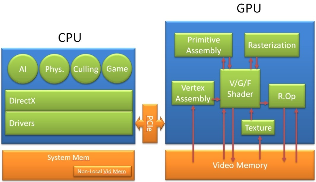
Fig. 70 From the GeForce 8 and 9 Series GPU Programming Guide (NVIDIA).

The surface of an object is drawn as a collection of triangles. The Application Programming Interface (API) is a standardized layer of software that allows an application (e.g.: a game) to send commands to a graphics processing unit to draw objects on a display. Examples of such APIs are DirectX and OpenGL. The host interface (the interface to the GPU) receives graphics commands and data from the CPU, communicates back the status and result data of the execution.

The two parts of a fixed function pipeline are shown in Fig. 71 and in Fig. 72.

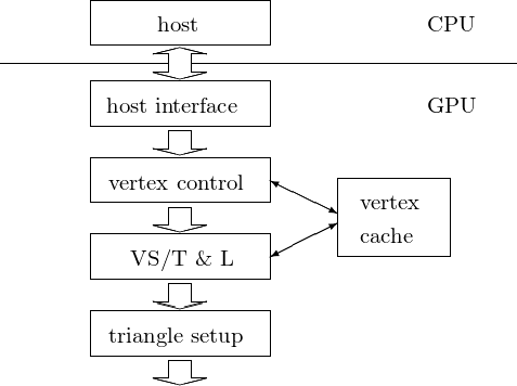
Fig. 71 Part one of a fixed function pipeline. VS/T & L = vertex shading, transform, and lighting.

The stages in the first part of the pipeline are as follows:

1. vertex control

   This stage receives parametrized triangle data from the CPU. The data gets converted and placed into the vertex cache.

2. VS/T & L (vertex shading, transform, and lighting)

   The VS/T & L stage transforms vertices and assigns per-vertex values, e.g.: colors, normals, texture coordinates, tangents. The vertex shader can assign a color to each vertex, but color is not applied to triangle pixels until later.

3. triangle setup

   Edge equations are used to interpolate colors and other per-vertex data across the pixels touched by the triangle.

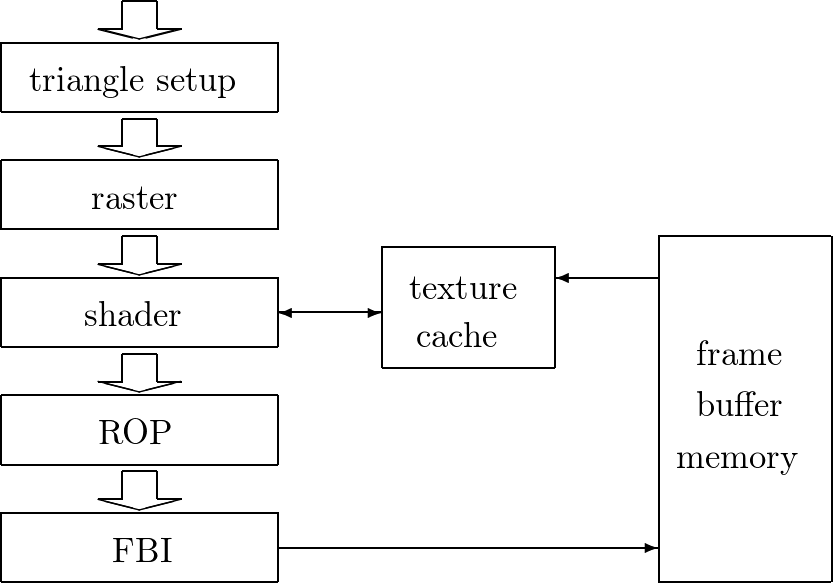
Fig. 72 Part two of a fixed-function pipeline. ROP = Raster Operation, FBI = Frame Buffer Interface

The stages in the second part of the pipeline are as follows:

4. raster

   The raster determines which pixels are contained in each triangle. Per-vertex values necessary for shading are interpolated.

5. shader

   The shader determines the final color of each pixel as a combined effect of interpolation of vertex colors, texture mapping, per-pixel lighting, reflections, etc.

6. ROP (Raster Operation)

   The final raster operations blend the color of overlapping/adjacent objects for transparency and antialiasing effects. For a given viewpoint, visible objects are determined and occluded pixels (blocked from view by other objects) are discarded.

7. FBI (Frame Buffer Interface)

   The FBI stages manages memory reads from and writes to the display frame buffer memory.

   For high-resolution displays, there is a very high bandwidth requirement in accessing the frame buffer. High bandwidth is achieved by two strategies: using special memory designs; and managing simultaneously multiple memory channels that connect to multiple memory banks.

Programmable Real-Time Graphics

Stages in graphics pipelines do many floating-point operations on completely independent data, e.g.: transforming the positions of triangle vertices, and generating pixel colors. This data independence as the dominating characteristic is the key difference between the design assumption for GPUs and CPUs. A single frame, rendered in 1/60-th of a second, might have a million triangles and 6 million pixels.

Vertex shader programs map the positions of triangle vertices onto the screen, altering their position, color, or orientation. A vertex shader thread reads a vertex position \((x,y,z,w)\) and computes its position on screen. Geometry shader programs operate on primitives defined by multiple vertices, changing them or generating additional primitives. Vertex shader programs and geometry shader programs execute on the vertex shader (VS/T & L) stage of the graphics pipeline.

A shader program calculates the floating-point red, green, blue, alpha (RGBA) color contribution to the rendered image at its pixel sample image position. The programmable vertex processor executes programs designated to the vertex shader stage. The programmable fragment processor executes programs designated to the (pixel) shader stage. For all graphics shader programs, instances can be run in parallel, because each works on independent data, produces independent results, and has no side effects. This property has motivated the design of the programmable pipeline stages into massively parallel processors.

An example of a programmable pipeline is illustrated by a schematic of a vertex processor in a pipeline, in Fig. 73 and by a schematic of a fragment processor in a pipeline, in Fig. 74.

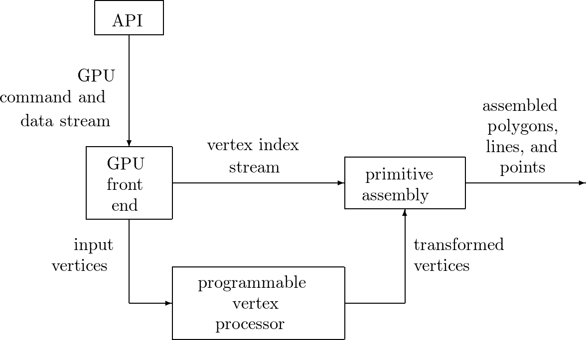
Fig. 73 A vertex processor in a pipeline.

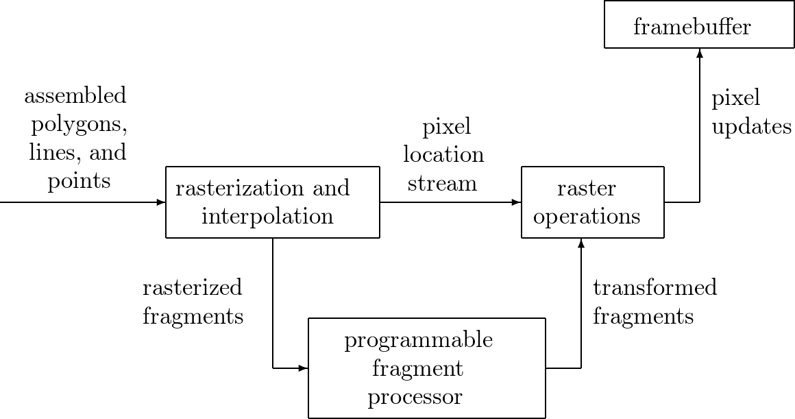
Fig. 74 A fragment processor in a pipeline.

Between the programmable graphics pipeline stages are dozens of fixed-function stages that perform well-defined tasks far more efficiently than a programmable processor could and which would benefit far less from programmability. For example, between the vertex processing stage and the pixel (fragment) processing stage is a rasterizer. The rasterizer — it does rasterization and interpolation — is a complex state machine that determines exactly which pixels (and portions thereof) lie within each geometric primitive’s boundaries. The mix of programmable and fixed-function stages is engineered to balance performance with user control over the rendering algorithm.

Introduced in 2006, the GeForce 8800 GPU mapped the separate programmable graphics stages to an array of unified processors. The graphics pipeline is physically a recirculating path that visits the processors three times, with much fixed-function tasks in between. More sophisticated shading algorithms motivated a sharp increase in the available shader operation rate, in floating-point operations. High-clock-speed design made programmable GPU processor array ready for general numeric computing. Original GPGPU programming used APIs (DirectX or OpenGL): to a GPU everything is a pixel.

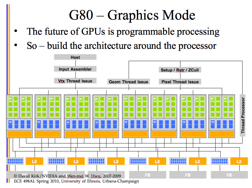
Fig. 75 GeForce 8800 GPU for GPGPU programming.

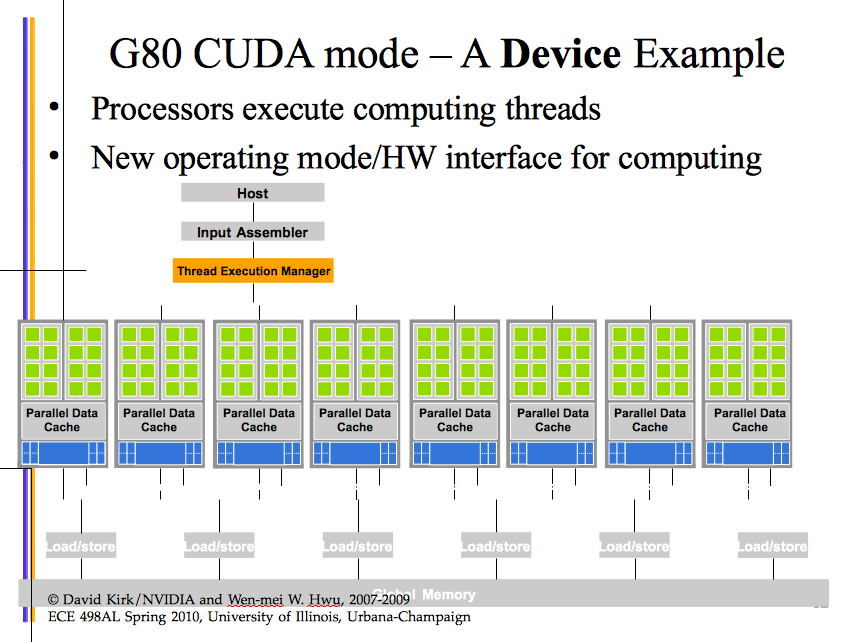
Fig. 76 GeForce 8800 GPU with new interface.

The drawbacks of the GPGPU model are many:

1. The programmer must know APIs and GPU architecture well.
2. Programs expressed in terms of vertex coordinates, textures, shader programs, add to the complexity.
3. Random reads and writes to memory are not supported.
4. No double precision is limiting for scientific applications.

Programming GPUs with CUDA (C extension): GPU computing.

Chapter 2 in the textbook ends mentioning the GT200. The next generation is code-named Fermi:

• 32 CUDA cores per streaming multiprocessor,
• 8 \(\times\) peak double precision floating point performance over GT200,
• true cache hierarchy, more shared memory,
• faster context switching, faster atomic operations.

We end this section with a number of figures about the GPU architecture, in Fig. 77, Fig. 78, and Fig. 79.

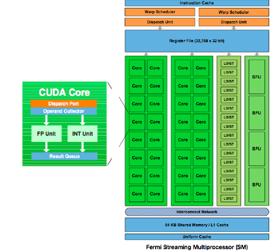
Fig. 77 The 3rd generation Fermi Architecture.

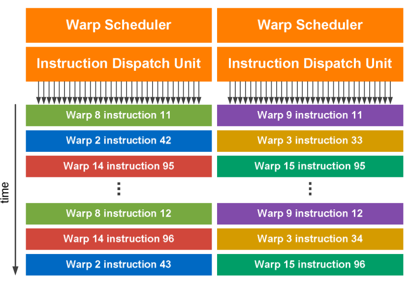
Fig. 78 Dual warp scheduler.

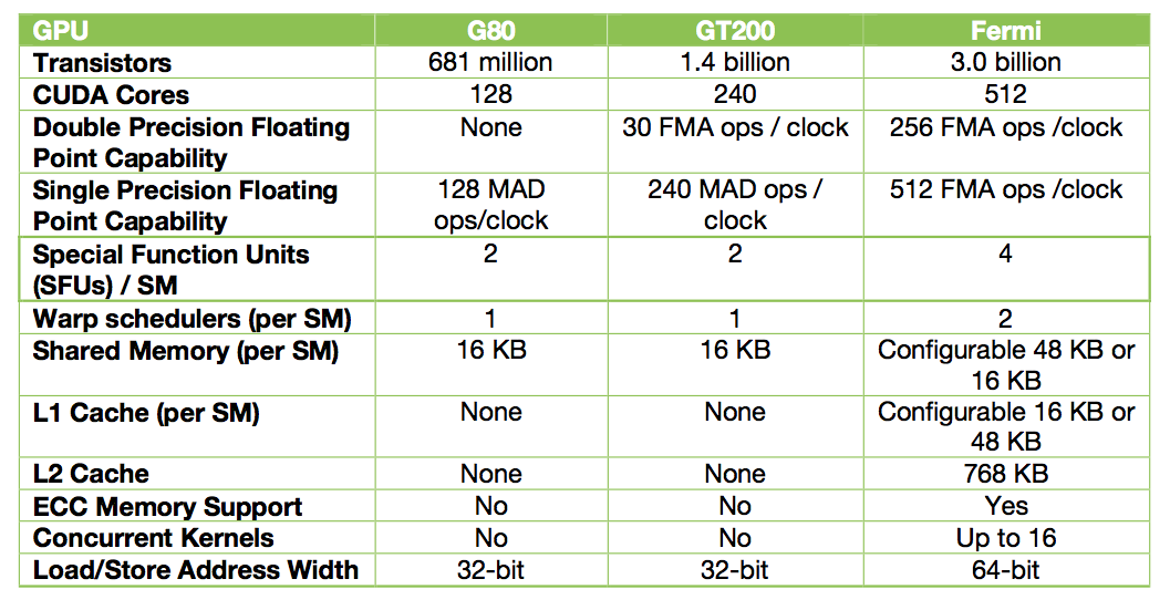
Fig. 79 Summary table of the GPU architecture.

The architecture of the NVIDIA Kepler GPU is summarized and illustrated in Fig. 80 and Fig. 81.

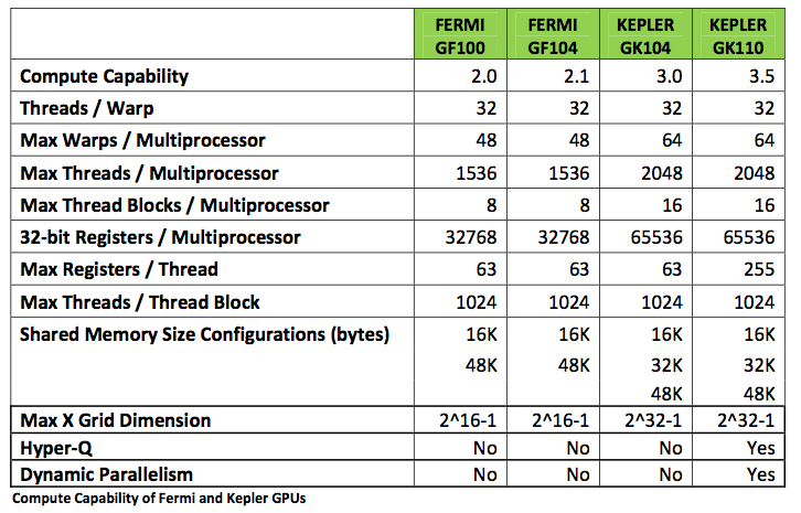
Fig. 80 The Kepler architecture.

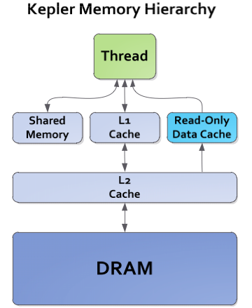
Fig. 81 Memory hierarchies of Kepler.

Summarizing this section, to fully utilize the GPU, one must use thousands of threads, whereas running thousands of threads on multicore CPU will swamp it. Data independence is the key difference between GPU and CPU.

Bibliography

Available at <http://www.nvidia.com>:

1. NVIDIA. Whitepaper NVIDIA’s Next Generation CUDA Compute Architecture: Fermi.
2. NVIDIA. Whitepaper NVIDIA’s Next Generation CUDA Compute Architecture: Kepler GK110.