Data Parallelism and Matrix Multiplication¶

Matrix multiplication is one of the fundamental building blocks in numerical linear algebra, and therefore in scientific computation. In this section, we investigate how data parallelism may be applied to solve this problem.

Data Parallelism¶

Many applications process large amounts of data. Data parallelism refers to the property where many arithmetic operations can be safely performed on the data simultaneously. Consider the multiplication of matrices \(A\) and \(B\) which results in \(C = A \cdot B\), with

\[A = [a_{i,j}] \in {\mathbb R}^{n \times m}, \quad B = [b_{i,j}] \in {\mathbb R}^{m \times p}, \quad C = [c_{i,j}] \in {\mathbb R}^{n \times p}.\]

\(c_{i,j}\) is the inner product of the i-th row of \(A\) with the j-th column of \(B\):

\[c_{i,j} = \sum_{k=1}^m a_{i,k} \cdot b_{k,j}.\]

All \(c_{i,j}\)‘s can be computed independently from each other. For \(n = m = p = 1,000\) we have 1,000,000 inner products. The matrix multiplication is illustrated in Fig. 88.

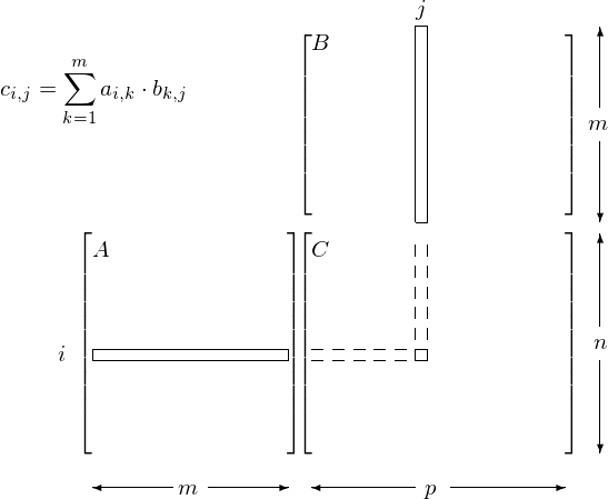
Fig. 88 Data parallelism in matrix multiplication.

Code for Matrix-Matrix Multiplication¶

Code for a device (the GPU) is defined in functions using the keyword __global__ before the function definition. Data parallel functions are called kernels. Kernel functions generate a large number of threads.

In matrix-matrix multiplication, the computation can be implemented as a kernel where each thread computes one element in the result matrix. To multiply two 1,000-by-1,000 matrices, the kernel using one thread to compute one element generates 1,000,000 threads when invoked.

CUDA threads are much lighter weight than CPU threads: they take very few cycles to generate and schedule thanks to efficient hardware support whereas CPU threads may require thousands of cycles.

A CUDA program consists of several phases, executed on the host: if no data parallelism, or on the device: for data parallel algorithms. The NVIDIA C compiler nvcc separates phases at compilation. Code for the host is compiled on host’s standard C compilers and runs as ordinary CPU process. device code is written in C with keywords for data parallel functions and further compiled by nvcc.

A CUDA program has the following structure:

CPU code
kernel<<<numb_blocks,numb_threads_per_block>>>(args)
CPU code

The number of blocks in a grid is illustrated in Fig. 89.

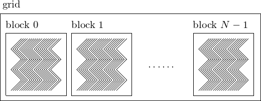
Fig. 89 The organization of the threads of execution in a CUDA program.

For the matrix multiplication \(C = A \cdot B\), we run through the following stages:

Allocate device memory for \(A\), \(B\), and \(C\).
Copy \(A\) and \(B\) from the host to the device.
Invoke the kernel to have device do \(C = A \cdot B\).
Copy \(C\) from the device to the host.
Free memory space on the device.

A linear address system is used for the 2-dimensional array. Consider a 3-by-5 matrix stored row-wise (as in C), as shown in Fig. 90.

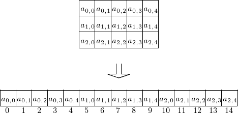
Fig. 90 Storing a matrix as a one dimensional array.

Code to generate a random matrix is below:

#include <stdlib.h>

__host__ void randomMatrix ( int n, int m, float *x, int mode )
/*
 * Fills up the n-by-m matrix x with random
 * values of zeroes and ones if mode == 1,
 * or random floats if mode == 0. */
{
   int i,j,r;
   float *p = x;

   for(i=0; i<n; i++)
      for(j=0; j<m; j++)
      {
         if(mode == 1)
            r = rand() % 2;
         else
            r = ((float) rand())/RAND_MAX;
         *(p++) = (float) r;
      }
}

The writing of a matrix is defined by the following code:

#include <stdio.h>

__host__ void writeMatrix ( int n, int m, float *x )
/*
 * Writes the n-by-m matrix x to screen. */
{
   int i,j;
   float *p = x;

   for(i=0; i<n; i++,printf("\n"))
      for(j=0; j<m; j++)
         printf(" %d", (int)*(p++));
}

In defining the kernel, we assign inner products to threads. For example, consider a 3-by-4 matrix \(A\) and a 4-by-5 matrix \(B\), as in Fig. 91.

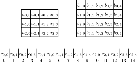
Fig. 91 Assigning inner products to threads.

The i = blockIdx.x*blockDim.x + threadIdx.x determines what entry in \(C = A \cdot B\) will be computed:

the row index in \(C\) is i divided by 5 and
the column index in \(C\) is the remainder of i divided by 5.

The kernel function is defined below:

__global__ void matrixMultiply
 ( int n, int m, int p, float *A, float *B, float *C )
/*
 * Multiplies the n-by-m matrix A
 * with the m-by-p matrix B into the matrix C.
 * The i-th thread computes the i-th element of C. */
{
   int i = blockIdx.x*blockDim.x + threadIdx.x;
   C[i] = 0.0;
   int rowC = i/p;
   int colC = i%p;
   float *pA = &A[rowC*m];
   float *pB = &B[colC];
   for(int k=0; k<m; k++)
   {
      pB = &B[colC+k*p];
      C[i] += (*(pA++))*(*pB);
   }
}

Running the program in a terminal window is shown below.

$ /tmp/matmatmul 3 4 5 1
a random 3-by-4 0/1 matrix A :
 1 0 1 1
 1 1 1 1
 1 0 1 0
a random 4-by-5 0/1 matrix B :
 0 1 0 0 1
 0 1 1 0 0
 1 1 0 0 0
 1 1 0 1 0
the resulting 3-by-5 matrix C :
 2 3 0 1 1
 2 4 1 1 1
 1 2 0 0 1
$

The main program takes four command line arguments: the dimensions of the matrices, that is: the number of rows and columns of \(A\), and the number of columns of \(B\). The fourth element is the mode, whether output is needed or not. The parsing of the command line arguments is below:

int main ( int argc, char*argv[] )
{
   if(argc < 4)
   {
      printf("Call with 4 arguments :\n");
      printf("dimensions n, m, p, and the mode.\n");
   }
   else
   {
      int n = atoi(argv[1]);    /* number of rows of A */
      int m = atoi(argv[2]);    /* number of columns of A */
                                /* and number of rows of B */
      int p = atoi(argv[3]);    /* number of columns of B */
      int mode = atoi(argv[4]); /* 0 no output, 1 show output */
      if(mode == 0)
         srand(20140331)
      else
         srand(time(0));

The next stage in the main program is the allocation of memories, on the host and on the device, as listed below:

float *Ahost = (float*)calloc(n*m,sizeof(float));
float *Bhost = (float*)calloc(m*p,sizeof(float));
float *Chost = (float*)calloc(n*p,sizeof(float));
randomMatrix(n,m,Ahost,mode);
randomMatrix(m,p,Bhost,mode);
if(mode == 1)
{
   printf("a random %d-by-%d 0/1 matrix A :\n",n,m);
   writeMatrix(n,m,Ahost);
   printf("a random %d-by-%d 0/1 matrix B :\n",m,p);
   writeMatrix(m,p,Bhost);
}
/* allocate memory on the device for A, B, and C */
float *Adevice;
size_t sA = n*m*sizeof(float);
cudaMalloc((void**)&Adevice,sA);
float *Bdevice;
size_t sB = m*p*sizeof(float);
cudaMalloc((void**)&Bdevice,sB);
float *Cdevice;
size_t sC = n*p*sizeof(float);
cudaMalloc((void**)&Cdevice,sC);

After memory allocation, the data is copied from host to device and the kernels are launched.

/* copy matrices A and B from host to the device */
cudaMemcpy(Adevice,Ahost,sA,cudaMemcpyHostToDevice);
cudaMemcpy(Bdevice,Bhost,sB,cudaMemcpyHostToDevice);

/* kernel invocation launching n*p threads */
matrixMultiply<<<n*p,1>>>(n,m,p,
                          Adevice,Bdevice,Cdevice);

/* copy matrix C from device to the host */
cudaMemcpy(Chost,Cdevice,sC,cudaMemcpyDeviceToHost);
/* freeing memory on the device */
cudaFree(Adevice); cudaFree(Bdevice); cudaFree(Cdevice);
if(mode == 1)
{
   printf("the resulting %d-by-%d matrix C :\n",n,p);
   writeMatrix(n,p,Chost);
}

Two Dimensional Arrays of Threads¶

Using threadIdx.x and threadIdx.y instead of a one dimensional organization of the threads in a block we can make the \((i,j)\)-th thread compute \(c_{i,j}\). The main program is then changed into

/* kernel invocation launching n*p threads */
dim3 dimGrid(1,1);
dim3 dimBlock(n,p);
matrixMultiply<<<dimGrid,dimBlock>>>
   (n,m,p,Adevice,Bdevice,Cdevice);

The above construction creates a grid of one block. The block has \(n \times p\) threads:

threadIdx.x will range between 0 and \(n-1\), and
threadIdx.y will range between 0 and \(p-1\).

The new kernel is then:

__global__ void matrixMultiply
 ( int n, int m, int p, float *A, float *B, float *C )
/*
 * Multiplies the n-by-m matrix A
 * with the m-by-p matrix B into the matrix C.
 * The (i,j)-th thread computes the (i,j)-th element of C. */
{
   int i = threadIdx.x;
   int j = threadIdx.y;
   int ell = i*p + j;
   C[ell] = 0.0;
   float *pB;
   for(int k=0; k<m; k++)
   {
      pB = &B[j+k*p];
      C[ell] += A[i*m+k]*(*pB);
   }
}

Examining Performance¶

Performance is often expressed in terms of flops.

1 flops = one floating-point operation per second;
use perf: Performance analysis tools for Linux
run the executable, with perf stat -e
with the events following the -e flag we count the floating-point operations.

For the Intel Sandy Bridge in kepler the codes are

530110 : FP_COMP_OPS_EXE:X87
531010 : FP_COMP_OPS_EXE:SSE_FP_PACKED_DOUBLE
532010 : FP_COMP_OPS_EXE:SSE_FP_SCALAR_SINGLE
534010 : FP_COMP_OPS_EXE:SSE_PACKED_SINGLE
538010 : FP_COMP_OPS_EXE:SSE_SCALAR_DOUBLE

Executables are compiled with the option -O2.

The performance of one CPU core is measured in the session below.

$ perf stat -e r530110 -e r531010 -e r532010 -e r534010 \
            -e r538010 ./matmatmul0 745 745 745 0

 Performance counter stats for './matmatmul0 745 745 745 0':

         1,668,710 r530110                                   [79.95%]
                 0 r531010                                   [79.98%]
     2,478,340,803 r532010                                   [80.04%]
                 0 r534010                                   [80.05%]
                 0 r538010                                   [80.01%]

       1.033291591 seconds time elapsed

Did 2,480,009,513 operations in 1.033 seconds: \(\Rightarrow (2,480,009,513/1.033)/(2^{30}) = 2.23 \mbox{GFlops}\).

The output of a session to measure the performance on the GPU, running matmatmul1 is below:

$ perf stat -e r530110 -e r531010 -e r532010 -e r534010 \
            -e r538010 ./matmatmul1 745 745 745 0

 Performance counter stats for './matmatmul1 745 745 745 0':

           160,925 r530110                                   [79.24%]
                 0 r531010                                   [80.62%]
         2,306,222 r532010                                   [80.07%]
                 0 r534010                                   [79.53%]
                 0 r538010                                   [80.71%]

       0.663709965 seconds time elapsed

The wall clock time is measured with the time command, as below:

$ time ./matmatmul1 745 745 745 0

real    0m0.631s
user    0m0.023s
sys     0m0.462s

The dimension 745 is too small for the GPU to be able to improve much. Let us thus increase the dimension.

$ perf stat -e r530110 -e r531010 -e r532010 -e r534010 \
            -e r538010 ./matmatmul0 4000 4000 4000 0

 Performance counter stats for './matmatmul0 4000 4000 4000 0':

        48,035,278 r530110                                  [80.03%]
                 0 r531010                                  [79.99%]
   267,810,771,301 r532010                                  [79.99%]
                 0 r534010                                  [79.99%]
                 0 r538010                                  [80.00%]

     171.334443720 seconds time elapsed

Now we will see if GPU acceleration leads to a speedup... The outcome accelerated performance measured is shown next:

$ perf stat -e r530110 -e r531010 -e r532010 -e r534010
            -e r538010 ./matmatmul1 4000 4000 4000 0

 Performance counter stats for './matmatmul1 4000 4000 4000 0':

           207,682 r530110                                  [80.27%]
                 0 r531010                                  [79.96%]
        64,222,441 r532010                                  [79.95%]
                 0 r534010                                  [79.94%]
                 0 r538010                                  [79.98%]

       1.011284551 seconds time elapsed

The speedup is 181.334/1.011 = 169, which is significant. Counting flops, f = 267,810,771,301

\(t_{\rm cpu} = 171.334\) and \(f/t_{\rm cpu}/(2^{30}) = 1.5\) GFlops.
\(t_{\rm gpu} = 1.011\) and \(f/t_{\rm gpu}/(2^{30}) = 246.7\) GFlops.

Exercises¶

Modify matmatmul0.c and matmatmul1.cu to work with doubles instead of floats. Examine the performance.
Modify matmatmul2.cu to use double indexing of matrices, e.g.: C[i][j] += A[i][k]*B[k][j].
Compare the performance of matmatmul1.cu and matmatmul2.cu, taking larger and larger values for \(n\), \(m\), and \(p\). Which version scales best?

Data Parallelism and Matrix Multiplication¶