Advanced MRI Reconstruction
an Application Case Study
Magnetic Resonance Imaging (MRI) is a safe and noninvasive probe of the structure and function of tissues in the body. MRI consists of two phases:
- Acquisition or scan: the scanner samples data in the spatial-frequency domain along a predefined trajectory.
- Reconstruction of the samples into an image.
The limitations of MRI are noise, imaging artifacts, long acquisition times. We have three often conflicting goals:
- Short scan time to reduce patient discomfort.
- High resolution and fidelity for early detection.
- High signal-to-noise ratio (SNR).
Massively parallel computing provides disruptive breakthrough.
Consider the the mathematical problem formulation. The reconstructed image \(m({\bf r})\) is
where
- \(W({\bf k})\) is the weighting function to account for nonuniform sampling;
- \(s({\bf k})\) is the measured k-space data.
The reconstruction is an inverse fast Fourier Transform on \(s({\bf k})\).
To reconstruct images, a Cartesian scan is slow and may result in poor images. A spiral scan of the data as shown schematically in Fig. 121 is faster and with gridding leads to images of better quality than the ones reconstructed in rectangular coordinates.
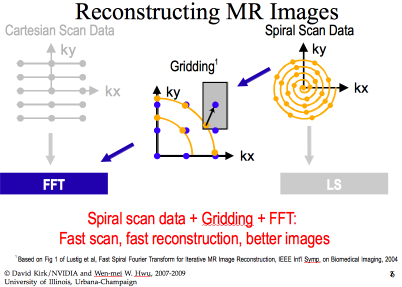
Fig. 121 A spiral scan of data to reconstruct images, LS = Least Squares.
The problem is summarized in Fig. 122, copied from the textbook of Hwu and Kirk.
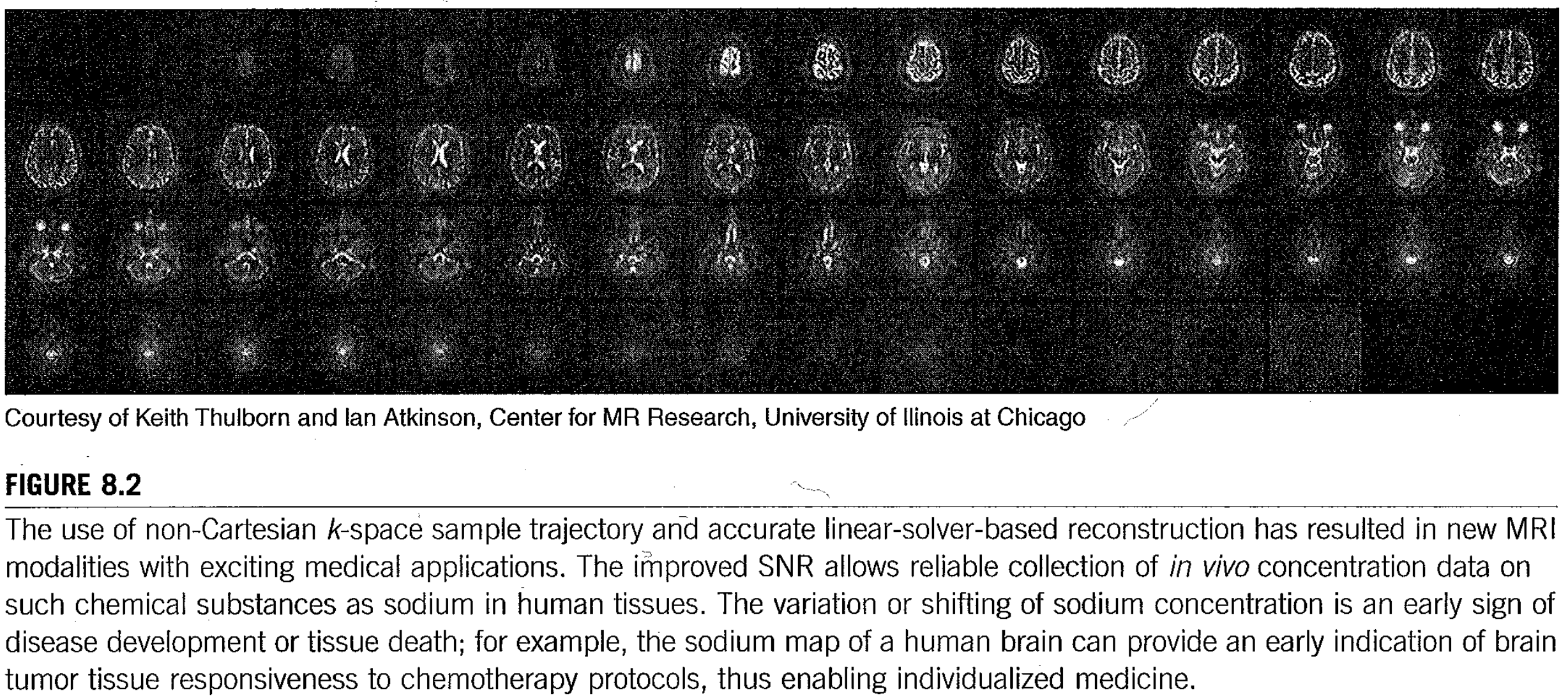
Fig. 122 Problem statement copied from Hwu and Kirk.
The mathematical problem formulation leads to an iterative reconstructiion method. We start with the formulation of a linear least squares problem, as a quasi-Bayesian estimation problem:
where
- \(\widehat{\rho}\) contains voxel values for reconstructed image,
- the matrix \({\bf F}\) models the imaging process,
- \({\bf d}\) is a vector of data samples, and
- the matrix \({\bf W}\) incorporates prior information, derived from reference images.
The solution to this linear least squares problem is
The advanced reconstruction algorithm consists of three primary computations:
\(\displaystyle Q({\bf x}_n) = \sum_{m=1}^M | \phi({\bf k}_m) |^2 e^{i 2 \pi {\bf k}_m \cdot {\bf x}_n}\)
where \(\phi(\cdot)\) is the Fourier transform of the voxel basis function.
\(\displaystyle \left[ {\bf F}^H {\bf d} \right]_n = \sum_{m=1}^M \phi^*({\bf k}_m) {\bf d}({\bf k}_m) e^{i 2\pi {\bf k}_m \cdot {\bf x}_m}\)
The conjugate gradient solver performs the matrix inversion to solve \(\left( {\bf F}^H {\bf F} + {\bf W}^H {\bf W} \right) \rho = {\bf F}^H {\bf d}\).
The calculation for \({\bf F}^H {\bf d}\) is an excellent candidate for acceleration on the GPU because of its substantial data parallelism.
Acceleration on a GPU
The computation of \({\bf F}^H {\bf d}\) is defined in the code below.
for(m = 0; m < M; m++)
{
   rMu[m] = rPhi[m]*rD[m] + iPhi[m]*iD[m];
   iMu[m] = rPhi[m]*iD[m] - iPhi[m]*rD[m];
   for(n = 0; n < N; n++)
   {
      expFHd = 2*PI*(kx[m]*x[n]
                   + ky[m]*y[n]
                   + kz[m]*z[n]);
      cArg = cos(expFHd);
      sArg = sin(expFHd);
      rFHd[n] += rMu[m]*cArg - iMu[m]*sArg;
      iFHd[n] += iMu[m]*cArg + rMu[m]*sArg;
   }
}
In the development of the kernel we consider the Compute to Global Memory Access (CGMA) ratio. A first version of the kernel follows:
__global__ void cmpFHd ( float* rPhi, iPhi, phiMag,
               kx, ky, kz, x, y, z, rMu, iMu, int N)
{
   int m = blockIdx.x*FHd_THREADS_PER_BLOCK + threadIdx.x;

   rMu[m] = rPhi[m]*rD[m] + iPhi[m]*iD[m];
   iMu[m] = rPhi[m]*iD[m] - iPhi[m]*rD[m];

   for(n = 0; n < N; n++)
   {
      expFHd = 2*PI*(kx[m]*x[n] + ky[m]*y[n] + kz[m]*z[n]);
      carg = cos(expFHd); sArg = sin(expFHd);
      rFHd[n] += rMu[m]*cArg - iMu[m]*sArg;
      iFHd[n] += iMu[m]*cArg + rMu[m]*sArg;
   }
}
A first modificiation is the splitting of the outer loop.
for(m = 0; m < M; m++)
{
   rMu[m] = rPhi[m]*rD[m] + iPhi[m]*iD[m];
   iMu[m] = rPhi[m]*iD[m] - iPhi[m]*rD[m];
}
for(m = 0; m < M; m++)
{
   for(n = 0; n < N; n++)
   {
      expFHd = 2*PI*(kx[m]*x[n]
                   + ky[m]*y[n]
                   + kz[m]*z[n]);
      cArg = cos(expFHd);
      sArg = sin(expFHd);
      rFHd[n] += rMu[m]*cArg - iMu[m]*sArg;
      iFHd[n] += iMu[m]*cArg + rMu[m]*sArg;
   }
}
We convert the first loop into a CUDA kernel:
__global__ void cmpMu ( float *rPhi,iPhi,rD,iD,rMu,iMu)
{
   int m = blockIdx * MU_THREADS_PER_BLOCK + threadIdx.x;

   rMu[m] = rPhi[m]*rD[m] + iPhi[m]*iD[m];
   iMu[m] = rPhi[m]*iD[m] - iPhi[m]*rD[m];
}
Because \(M\) can be very big, we will have many threads. For example, if \(M = 65,536\), with 512 threads per block, we have \(65,536/512 = 128\) blocks.
Then the second loop is defined by another kernel.
__global__ void cmpFHd ( float* rPhi, iPhi, PhiMag,
             kx, ky, kz, x, y, z, rMu, iMu, int N )
{
   int m = blockIdx.x*FHd_THREADS_PER_BLOCK + threadIdx.x;

   for(n = 0; n < N; n++)
   {
      float expFHd = 2*PI*(kx[m]*x[n]+ky[m]*y[n]
                                     +kz[m]*z[n]);
      float cArg = cos(expFHd);
      float sArg = sin(expFHd);

      rFHd[n] += rMu[m]*cArg - iMu[m]*sArg;
      iFHd[n] += iMu[m]*cArg + rMu[m]*sArg;
   }
}
To avoid conflicts between threads, we interchange the inner and the outer loops:
for(m=0; m<M; m++)                for(n=0; n<N; n++)
{                                 {
   for(n=0; n<N; n++)                for(m=0; m<M; m++)
   {                                 {
      expFHd = 2*PI*(kx[m]*x[n]         expFHd = 2*PI*(kx[m]*x[n]
                    +ky[m]*y[n]                       +ky[m]*y[n]
                    +kz[m]*z[n]);                     +ky[m]*y[n]);
      cArg = cos(expFHd);               cArg = cos(expFHd);
      sArg = sin(expFHd);               sArg = sin(expFHd);
      rFHd[n] += rMu[m]*cArg            rFHd[n] += rMu[m]*cArg
               - iMu[m]*sArg;                    - iMu[m]*sArg;
      iFHd[n] += iMu[m]*cArg            rFHd[n] += iMu[m]*cArg
               + rMu[m]*sArg;                    + rMu[m]*sArg;
   }                                 }
}                                 }
In the new kernel, the n-th element will be computed
by the n-th thread. The new kernel is listed below.
__global__ void cmpFHd ( float* rPhi, iPhi, phiMag,
             kx, ky, kz, x, y, z, rMu, iMu, int M )
{
   int n = blockIdx.x*FHD_THREAD_PER_BLOCK + threadIdx.x;

   for(m = 0; m < M; m++)
   {
      float expFHd = 2*PI*(kx[m]*x[n]+ky[m]*y[n]
                                     +kz[m]*z[n]);
      float cArg = cos(expFHd);
      float sArg = sin(expFHd);
      rFHd[n] += rMu[m]*cArg - iMu[m]*sArg;
      iFHd[n] += iMu[m]*cArg + rMu[m]*sArg;
   }
}
For a \(128^3\) image, there are \((2^7)^3 = 2,097,152\) threads. For higher resolutions, e.g.: \(512^3\), multiple kernels may be needed.
To reduce memory accesses, the next kernel uses registers:
__global__ void cmpFHd ( float* rPhi, iPhi, phiMag,
             kx, ky, kz, x, y, z, rMu, iMu, int M )
{
   int n = blockIdx.x*FHD_THREAD_PER_BLOCK + threadIdx.x;
   float xn = x[n]; float yn = y[n]; float zn = z[n];
   float rFHdn = rFHd[n]; float iFHdn = iFHd[n];
   for(m = 0; m < M; m++)
   {
      float expFHd = 2*PI*(kx[m]*xn+ky[m]*yn+kz[m]*zn);
      float cArg = cos(expFHd);
      float sArg = sin(expFHd);
      rFHdn += rMu[m]*cArg - iMu[m]*sArg;
      iFHdn += iMu[m]*cArg + rMu[m]*sArg;
   }
   rFHd[n] = rFHdn; iFHd[n] = iFHdn;
}
The usage of registers improved the Compute to Memory Access (CGMA) ratio.
Using constant memory we use cache more efficiently. The technique is called chunking data. Limited in size to 64KB, we need to invoke the kernel multiple times.
__constant__ float kx[CHUNK_SZ],ky[CHUNK_SZ],kz[CHUNK_SZ];
// code omitted ...
for(i = 0; k < M/CHUNK_SZ; i++)
{
   cudaMemcpy(kx,&kx[i*CHUNK_SZ],4*CHUNK_SZ,
              cudaMemCpyHostToDevice);
   cudaMemcpy(ky,&ky[i*CHUNK_SZ],4*CHUNK_SZ,
              cudaMemCpyHostToDevice);
   cudaMemcpy(kz,&kz[i*CHUNK_SZ],4*CHUNK_SZ,
              cudaMemCpyHostToDevice);
   // code omitted ...
   cmpFHD<<<FHd_THREADS_PER_BLOCK,
            N/FHd_THREADS_PER_BLOCK>>>
     (rPhi,iPhi,phiMag,x,y,z,rMu,iMu,M);
}
Due to size limitations of constant memory and cache, we will adjust the memory layout. Instead of storing the components of k-space data in three separate arrays, we use an array of structs:
struct kdata
{
   float x, float y, float z;
}
__constant struct kdata k[CHUNK_SZ];
and then in the kernel
we use k[m].x, k[m].y, and k[m].z.
In the next optimization, we use the hardware trigonometric functions.
Instead of cos and sin as implemented in software,
the hardware versions __cos and __sin provide
a much higher throughput.
The __cos and __sin are implemented as hardware
instructions executed by the special function units.
We need to be careful about a loss of accuracy.
The validation involves a perfect image:
- a reverse process to generate scanned data;
- metrics: mean square error and signal-to-noise ratios.
The last stage is the experimental performance tuning.
Bibliography
- A. Lu, I.C. Atkinson, and K.R. Thulborn. Sodium Magnetic Resonance Imaging and its Bioscale of Tissue Sodium Concentration. Encyclopedia of Magnetic Resonance, John Wiley and Sons, 2010.
- S.S. Stone, J.P. Haldar, S.C. Tsao, W.-m.W. Hwu, B.P. Sutton, and Z.-P. Liang. Accelerating advanced MRI reconstructions on GPUs. Journal of Parallel and Distributed Computing 68(10): 1307-1318, 2008.
- The IMPATIENT MRI Toolset, open source software available at <http://impact.crhc.illinois.edu/mri.php>.