Mixed Subdivisions of Newton Polytopes to compute Mixed Volumes

For (2), we collect the exponent vectors of the system P in the supports $\cal A$:

$$\begin{array}{l} P(x_1,x_2) = \\ ~~~~~ \left\{ \begin{a... ...,0) \} \\ ~~~~ A_2 = \{ (0,0) , (1,2) , (3,1) \} \end{array}$$ (15)

The supports A₁ and A₂ span the respective Newton polytopes Q₁ and Q₂.

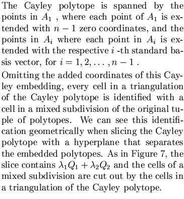
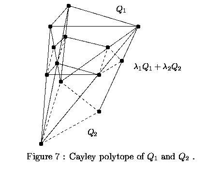
The Cayley trick [33, Proposition 1.7, page 274] is a method to rewrite a certain resultant as a discriminant of one single polynomial with additional variables. The polyhedral version of this trick as in [102, Lemma 5.2] is due to Bernd Sturmfels. It provides a one-to-one correspondence between the cells in a mixed subdivision and a triangulation of the so-called Cayley polytope spanned by the points of A_i embedded in a (2n-1)-dimensional space. See [45] for another application besides mixed-volume computation. As in [45], Figure 7 gives a ``one-picture proof'' of this trick, displaying the Cayley polytope for the supports $\cal A$in (15). Note that this construction provides a definition for mixed subdivisions.

 $\parbox{8cm}{ \par The Cayley polytope is spanned by the points in $... ...sion are cut out by the cells in a triangulation of the Cayley polytope. \par }$  $\parbox{10cm}{ \begin{center} \centerline{\psfig{figure=psfcayley.ps... ...polytope of $Q_1$\space and $Q_2$ . \addtocounter{figure}{1} \end{center}\par }$

The Cayley trick was implemented in [112] as an application of the dynamic lifting algorithm to construct regular triangulations. This method calculates the volume polynomial (4) completely. When one is only interested in the mixed volume, the method is only efficient when the supports do not differ much from each other.

To compute only the mixed volume, the lift-and-prune approach was presented in [24], using a primal model to prune in the tree of edge-edge combinations. This approach operates in two stages. First the polytopes are lifted by adding one coordinate to every point in the supports. In the second stage, one computes the facets of the lower hull of the Minkowski sum that are spanned by sums of edges. These facets constitute the mixed cells in a mixed subdivision. On the supports $\cal A$ in (15), we consider the lifted supports

$${\widehat {\cal A}} = ({\widehat A}_1,{\widehat A}_2) \quad... ...widehat A}_2 = \{ (0,0,0) , (1,2,0) , (3,1,1) \} \end{array}$$ (16)

The lower hulls of the lifted polytopes are displayed in Figure 8.

  

Figure: Lifted polytopes ${\widehat Q}_1$, ${\widehat Q}_2$, and a regular mixed subdivision of ${\widehat Q}_1 + {\widehat Q}_2$.

The two cells that contribute to the mixed volume are identified by inner normals $\alpha$ and $\beta$ that satisfy systems of linear equations and inequalities:

$$\begin{array}{l} \! \! \! \! \alpha = (0,0,1) \\ \left\{... ...& < & 3 \beta_1 + \beta_2 + 1 \end{array} \right. \end{array}$$ (17)

These systems express that the cells correspond to facets spanned by the sum of two edges on the lower hulls of ${\widehat Q}_1$ and ${\widehat Q}_2$ respectively. The lift-and-prune method with a dual version of the linear inequality constrains as in (17) was elaborated in [112], exploiting the fact that several polynomials can share the same Newton polytope (see [40]) and with dimension reductions.

The geometric dual construction to Figure 8 is displayed in Figure 9.

  

Figure: On the left we see the projection of a regular mixed subdivision of ${\widehat Q}_1 + {\widehat Q}_2$. On the right, we have the dual construction with complexes ${\cal N}_{\vee}^{1}(Q_1)$ and ${\cal N}_{\vee}^{1}(Q_2)$collecting the cones of all vectors normal to the edges on the lower hulls of ${\widehat Q}_1$ and ${\widehat Q}_2$ respectively. The intersection of the cones contain the normals to the mixed cells.

As in [40], we assume that there are r different Newton polytopes. Given a tuple of lifted point sets ${\widehat {\cal A}} = ( {\widehat A}_1, {\widehat A}_2, \ldots, {\widehat A}_r )$, any lifted cell ${\widehat {\cal C}}_{\bf v}$ of a regular subdivision can be characterized by its inner normal as

$${\widehat {\cal C}}_{\bf v} = ( \partial_{\bf v} {\widehat A... ...} {\widehat A}_2, \ldots , \partial_{\bf v} {\widehat A}_r ).$$ (18)

Since ${\rm conv}({\widehat C}_{\bf v}) = {\rm conv}(\sum_{i=1}^r \partial_{\bf v} {\widehat A}_i)$ is a facet of the lower hull, the inner product $\langle . , {\bf v} \rangle$ attains
its minimum over ${\widehat A}_i$ at $\partial_{\bf v} {\widehat A}_i$, i.e.,

$$\forall {\widehat {\bf a}}, {\widehat {\bf b}} \in \partia... ... {\widehat {\bf b}} , {\bf v} \rangle, \quad i = 1,2,\ldots,r,$$ (19)

$$\forall {\widehat {\bf a}} \in {\widehat A}_i \setminus \p... ... {\widehat {\bf b}} , {\bf v} \rangle, \quad i = 1,2,\ldots,r.$$ (20)

Algorithm 5.1 (presented in [112]) gives a way to compute all mixed cells by searching for feasible solutions to the constraints (19) and (20). The algorithm generates a tree of all possible combinations of k_i-faces, with feasibility tests to prune branches that do not lead to mixed cells. The order of enumeration is organized so that mixed cells which share some faces also share a part of the factorization work to be done to solve the system defined by (19).

Algorithm 5.1   Pruning algorithm with shared factorizations subject to inequality constraints:

Input: $({\widehat A}_1,{\widehat A}_2, \ldots, {\widehat A}_r)$,

lifted point sets

$\!$ ${\bf k} = (k_1,k_2,\ldots,k_r)$, $n = \sum_{i=1}^r k_i$,

A_i appears k_i times

$\!$ $({\widehat {\cal F}}_1,{\widehat {\cal F}}_2, \ldots, {\widehat {\cal F}}_r)$.

k_i-faces of lower hull of ${\rm conv}({\widehat A}_i)$

Output: ${\widehat {\frak S}_\omega} = \{ \ {\widehat {\cal C}} \in {\widehat S}_\omega \ \vert \ V_n({\cal C},{\bf k}) > 0 \ \}$.

collection of lifted mixed cells

At level i, $1 \leq i < r$:

DATA and INVARIANT CONDITIONS:

$\!$ $(M_1,\kappa)$: $M_1 {\bf v} = {\bf0} \not\Rightarrow v_{n+1} = 0$, $\kappa = {\displaystyle \sum_{j=1}^{i-1} k_j}$

equalities (19)

upper triangular up to row $\kappa$

$(M_2,\kappa)$:	$M_2 {\bf v} \geq {\bf0} \not\Rightarrow -v_{n+1} \geq 0$
	$\dim(M_2) = n-\kappa$

inequalities (20)

still feasible and reduced

ALGORITHM:

for each ${\widehat C}_i \in {\widehat {\cal F}}_i$ loop

enumerate over all k_i-faces

Triangulate $(M_1,\kappa,{\widehat C}_i)$;

ensure invariant conditions

if $M_1 {\bf v} = {\bf0} \not\Rightarrow v_{n+1} = 0$

test for feasibility w.r.t. (19)

then Eliminate $(M_1,M_2,\kappa,{\widehat C}_i, {\widehat A}_i)$;

eliminate unknowns

if $M_2 {\bf v} \geq {\bf0} \not\Rightarrow -v_{n+1} \geq 0$

test for feasibility w.r.t. (20)

then proceed to next level i+1;

end if;

end if;

end for.

At level i=r:

Compute $\bf v$: $M_1 {\bf v} = {\bf0}$;

Merge the new cell ${\cal C}_{\bf v}$ with the list ${\widehat {\frak S}_\omega}$.

Note that (20) has to be weakened to $\geq$ type inequalities in order to be able to compute also subdivisions that are not fine. This also explains the merge operation at the end. The feasibility tests in the algorithm allow an efficient computation of the mixed cells. The conditions (19) and (20) are verified incrementally. After choosing a k_i-face ${\widehat C}_i = \{ {\widehat {\bf c}}_{0i}, {\widehat {\bf c}}_{1i} , \ldots , {\widehat {\bf c}}_{k_i i} \}$ of ${\widehat A}_i$, linear programming is used to check whether $({\widehat C}_1, \ldots , {\widehat C}_i )$can lead to a mixed cell in the induced subdivision.

We end this section with complexity results. The complexity of computing mixed volumes is proven [21] to be $\char93 P$-hard. This complexity class is typical for all enumerative problems, since, unlike the class NP, there exists no algorithm that runs in polynomial time for arbitrary dimensions to verify that a guessed answer is correct. Although the current algorithmical practice suggests that computing mixed volumes is harder than computing volumes of polytopes (which is also known as a $\char93 P$-hard problem [20]), this is not the case from a complexity point of view as shown in [21]. In [25] it is shown that the mixed volume  $V_n({\cal Q})$ is bounded from below by $n! {\rm vol}_n(Q_\mu)$, $Q_\mu$ being the polytope of minimum volume in ${\cal Q}$.